Triage#

Predictive analytics projects require coordinating many tasks, such as feature generation, classifier training, evaluation, and list generation. Each of these tasks is complicated in its own right, but it also needs to be combined with the other tasks throughout the course of the project.

DSaPP built triage to facilitate the creation of supervised learning models, in particular binary classification models with a strong temporal component in the data.

The dataset's temporal component mainly affects two modeling steps: feature creation (you need to be careful to avoid leaking information from the future through your features) and hyperparameter selection. triage solves both by splitting the data into temporal blocks and automating temporal cross-validation (TCC) and the feature generation.

triage uses the concept of an experiment. An experiment consists of a series of steps that aim to generate a good model for predicting the label of an entity in the data set. The steps are data time-splitting, label generation, feature generation, matrix creation, model training, predictions, and model evaluation. In each of these steps, triage will handle the temporal nuances of the data.

Nowadays triage will help you to select the best model (model selection) and it allows you to explore and understand the behavior of your models using post-modeling techniques.

You need to specify (via a configuration file) how you want to split your data temporally, which combination of machine learning algorithms and their hyperparameters you'd like to use, which kinds of features you want to generate, which subsets of those features you want to try in each model, and which metrics you'd like to use to evaluate performance and provide some criteria to select the best model.

An experiment run consists in fitting every combination of algorithm, hyperparameters, and feature subsets to the temporally split data and evaluating their predictive performance on future data splits using the user's metrics.

triage calls a unique combination of algorithm, hyperparameters, and feature subsets a model_group and a model group fit to a specific data matrix a model. Our data typically span multiple time periods, so triage fits multiple models for each model group.

triage is simple to use, but it contains a lot of complex concepts that we will try to clarify in this section. First we will explain how to run triage, and then we will create a toy experiment that helps explain triage's main concepts.

Triage interface#

To run a triage experiment, you need the following:

A database with the data that you want to model.
- In this tutorial, the credentials are part of the DATABASE_URL environment variable
triage installed in your environment. You can verify that triage is indeed installed if you type in bastion:

triage -h

An experiment config file. This is where the magic happens. We will discuss this file at length in this section of the tutorial.

We are providing a docker container, bastion, that executes triage experiments. You already had the database (you were working on it the last two sections of this tutorial, remember?). So, like a real project, you just need to worry about the experiment configuration file.

In the following section of the tutorial we will use a small experiment configuration file located at <../triage/experiments/simple_test_skeleton.yaml>.

We will show you how to setup the experiment while explaining the inner workings of triage. We will modify the configuration file to show the effects of the configuration parameters. If you want to follow along, we suggest you copy that file and modify by yourself.

You can run that experiment with:

# Remember to run this in bastion NOT in your laptop!
triage experiment experiments/simple_test_skeleton.yaml

Every time you modify the configuration file and see the effects, you should execute the experiment again using the previous command.

A simple `triage` experiment#

A brief recap of Machine Learning#

Triage helps you to run a Machine learning experiment. An experiment in this context means the use of Machine Learning to explore a dynamic system in order to do some predictions about it.

Before execute the any ML experiment, you need to define some boundaries:

Which are the entities that you want to study?
What will you want to know about them?

In DSaPP, we build ML systems that aim to have social impact, i.e. help government offices, NGOs or other agents to do their job better. "Do their job better" means increase their reach (e.g. identify correctly more entities with some characteristics) using more efficiently their (scarce) resources (e.g. inspectors, medics, money, etc).

With this optic, the boundaries are:

Cohort: Which are the entities that you want to reach?
Label: What will you want to know about them?
Label timespan: In what time period?
Update frequency: How frequently do you want to intervene?
List size: How many resources do you have to intervene?

Triage's experiment configuration file structures this information.

Cohorts, labels, event dates and as of dates#

We will use the inspections prioritization as a narrative to help clarify these concepts:

Which are the entities that you want to reach?*: Active facilities, i.e. facilities that exists at the day of the *planning inspections. We don't want to waste city resources (inspectors time) going to facilities that are out of business.
What will you want to know about them?: Will those facilities fail the inspection?
In what time period?: Will those facilities fail the inspection in the following month?
How frequently do you want to intervene?: Every month.
How many resources do you have to intervene?: We only have one inspector, so, one inspection per month

To exemplify and explain the inner workings of triage in this scenario, we will use a subset of the semantic.events table with the following facilities (i.e. imagine that Chicago only has this three facilities):

select
    entity_id,
    license_num,
    facility_aka,
    facility_type,
    activity_period
from
    semantic.entities
where
    license_num in (1596210, 1874347, 1142451)
order by
    entity_id asc;

entity_id	license_num	facility_aka	facility_type	activity_period
229	1596210	food 4 less	grocery store	[2010-01-08,)
355	1874347	mcdonalds	restaurant	[2010-01-12,2017-11-09)
840	1142451	jewel foodstore # 3345	grocery store	[2010-01-26,)

The first thing triage does when executes the experiment, is split the time that the data covers in blocks considering the time horizon for the label ( Which facilities will fail an inspection in the following month? in this scenario of inspection prioritization¹) . This time horizon is calculated from a set of specific dates (as_of_date in triage parlance) that divide the blocks in past (for training the model) and future (for testing the model). The set of as_of_dates is (mainly) calculated from the label timespan and the update frequency². The as of date is not the event date. The event date occurred when the facility was inspected. The as of date is when the planning of the future facilities to be inspected happens.

triage will create those labels using information about the outcome of the event³, taking into account the temporal structure of the data. In our example: if a facility is inspected is an event, and whether it fails the inspection (outcome true) or not (outcome false).

For a given entity on a given as of date, triage asks whether there's an outcome in the future time horizon. If so, triage will generate a label for that specific entity on that as of date.

For this example, the label will be if given an as of date (e.g. January first, 2014), the facility will have a failed inspection in the following year.

The following example hopefully will clarify the difference between outcome and label. We will focus on events (inspections) that happened in the year of 2014.

select
    date,
    entity_id,
    (result = 'fail') as outcome
from
    semantic.events
where
    '[2014-01-01, 2015-01-01]'::daterange @> date
    and
    entity_id in (229,355,840)
order by
    date asc;

date	entity_id	outcome
2014-01-14	840	f
2014-02-04	229	f
2014-02-24	840	t
2014-03-05	840	f
2014-04-10	355	t
2014-04-15	229	f
2014-04-18	355	f
2014-05-06	840	f
2014-08-28	355	f
2014-09-19	229	f
2014-09-30	355	t
2014-10-10	355	f
2014-10-31	840	f

We can observe that the facilities had several inspections, but in that timeframe 362 y 859 had failed inspections.

Continuing the narrative, from the perspective of the day of 2014-01-01 (as of date), those facilities will have positive label.

We can express that in a query and getting the labels for that as of date :

select
    '2014-01-01' as as_of_date,
    entity_id,
    bool_or(result = 'fail')::integer as label
from
    semantic.events
where
    '2014-01-01'::timestamp <= date
    and date < '2014-01-01'::timestamp + interval '1 year'
    and entity_id in (229,355,840)
group by
    entity_id;

as_of_date	entity_id	label
2014-01-01	229	0
2014-01-01	355	1
2014-01-01	840	1

Note that ee transform the label to integer, since the machine learning algorithms only work with numeric data.

We also need a way to store the state of each entity. We can group entities in cohorts defined by the state. The cohort can be used to decide which facilities you want to predict on (i.e. include in the ML train/test matrices). The rationale of this comes from the need to only predict for entities in a particular state: Is the restaurant new? Is this facility on this zip code? Is the facility "active"?⁴

We will consider a facility as active if a given as of date is in the interval defined by the start_date and end_date.

select
    '2018-01-01'::date as as_of_date,
    entity_id,
    activity_period,
case when
activity_period @> '2018-01-01'::date -- 2018-01-01 is as of date
then 'active'::text
else 'inactive'::text
end as state
from
    semantic.entities
where
    entity_id in (229,355,840);

as_of_date	entity_id	activity_period	state
2018-01-01	229	[2010-01-08,)	active
2018-01-01	355	[2010-01-12,2017-11-09)	inactive
2018-01-01	840	[2010-01-26,)	active

Triage will use a simple modification of the queries that we just discussed for automate the generation of the cohorts and labels for our experiment.

Experiment configuration file#

The experiment configuration file is used to create the experiment object. Here, you will specify the temporal configuration, the features to be generated, the labels to learn, and the models that you want to train in your data.

The configuration file is a yaml file with the following main sections:

temporal_config: Temporal specification of the data, used for creating the blocks for temporal crossvalidation.
cohort_config: Using the state of the entities, define (using sql) cohorts to filter out objects that shouldn't be included in the training and prediction stages. This will generate a table call cohort_{experiment_hash}
label_config: Specify (using sql) how to generate labels from the event's outcome. A table named labels_{experiment_hash} will be created.
feature_aggregation: Which spatio-temporal aggregations of the columns in the data set do you want to generate as features for the models?
model_group_keys: How do you want to identify the model_group in the database (so you can run analysis on them)?
grid_config: Which combination of hyperparameters and algorithms will be trained and evaluated in the data set?
scoring: Which metrics will be calculated?

Two of the more important (and potentially confusing) sections are temporal_config and feature_generation. We will explain them in detail in the next sections.

Temporal crossvalidation#

Cross validation is a common technique to select a model that generalizes well to new data. Standard cross validation randomly splits the training data into subsets, fits models on all but one, and calculates the metric of interest (e.g. precision/recall) on the one left out, rotating through the subsets and leaving each out once. You select the model that performed best across the left-out sets, and then retrain it on the complete training data.

Unfortunately, standard cross validation is inappropriate for most real-world data science problems. If your data have temporal correlations, standard cross validation lets the model peek into the future, training on some future observations and testing on past observations. To avoid this problem, you should design your training and testing to mimic how your model will be used, making predictions only using the data that would be available at that time (i.e. from the past).

In temporal crossvalidation, rather than randomly splitting the dataset into training and test splits, temporal cross validation splits the data by time.

triage uses the timechop library for this purpose. Timechop will "chop" the data set in several temporal blocks. These blocks are then used for creating the features and matrices for training and evaluation of the machine learning models.

Assume we want to select which restaurant (of two in our example dataset) we should inspect next year based on its higher risk of violating some condition. Also assume that the process of picking which facility is repeated every year on January 1^st⁵

Following the problem description template given in Section Description of the problem to solve, the question that we'll attempt to answer is:

Which facility ( $n=1$ ) is likely to violate some inspected condition in the following year ( $X=1$ )?

The traditional approach in machine learning is splitting the data in training and test datasets. Train or fit the algorithm on the training data set to generate a train model and test or evaluate the model on the test data set. We will do the same here, but, with the help of timechop we will take in account the time:

We will fit models on training set up to 2014-01-01 and see how well those models would have predicted 2015; fit more models on training set up to 2015-01-01 and see how well those models would have predicted 2016; and so on. That way, we choose models that have historically performed best at our task, forecasting. It’s why this approach is sometimes called evaluation on a rolling forecast origin because the origin at which the prediction is made rolls forward in time. ⁶

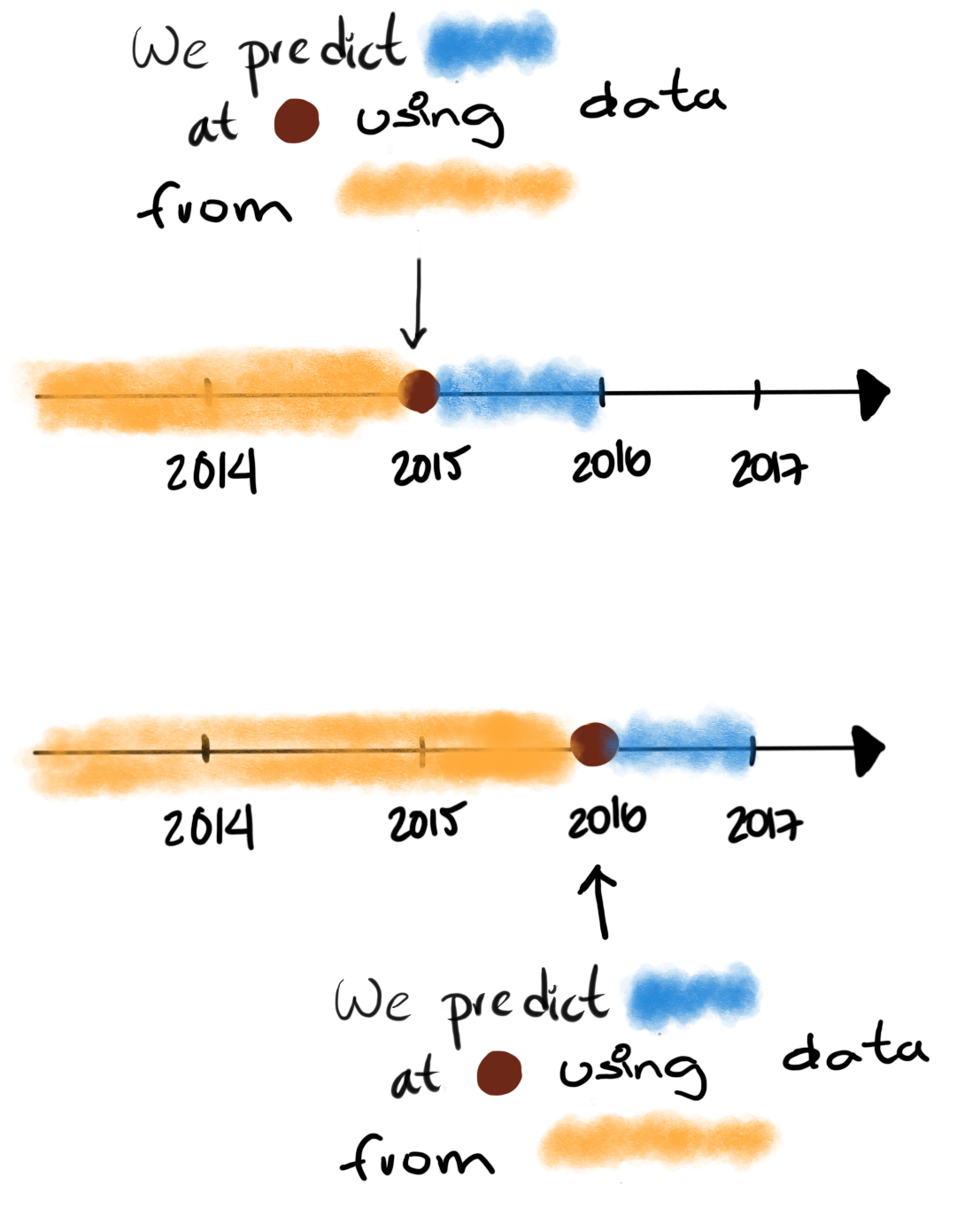
The data at which the model will do the predictions is denominated as as of date in triage (as of date = January first in our example). The length of the prediction time window (1 year) is called label span. Training and predicting with a new model as of date (every year) is the model update frequency.

Because it's inefficient to calculate by hand all the as of dates or prediction points, timechop will take care of that for us. To do so, we need to specify some more constraints besides the label span and the model update frequency:

What is the date range covered by our data?
What is the date range in which we have information about labels?
How frequently do you receive information about your entities?
How far in the future you want to predict?
How much of the past data do you want to use?

With this information, timechop will calculate as-of train and test dates from the last date in which you have label data, using the label span in both test and train sets, plus the constraints just mentioned.

In total timechop uses 11 configuration parameters⁷.

There are parameters related to the boundaries of the available data set:
- feature_start_time: data aggregated into features begins at this point (earliest date included in features)
- feature_end_time: data aggregated into features is from before this point (latest date included in features)
- label_start_time: data aggregated into labels begins at this point (earliest event date included in any label (event date >= label_start_time)
- label_end_time: data aggregated is from before this point (event date < label_end_time to be included in any label)
Parameters that control the labels' time horizon on the train and test sets:
- training_label_timespans: how much time is covered by training labels (e.g., outcomes in the next 3 days? 2 months? 1 year?) (training prediction span)
- test_label_timespans: how much time is covered by test prediction (e.g., outcomes in the next 3 days? 2 months? 1 year?) (test prediction span)
These parameters will be used with the outcomes table to generate the labels. In an early warning setting, they will often have the same value. For inspections prioritization, this value typically equals test_durations and model_update_frequency.
Parameters related about how much data we want to use, both in the future and in the past relative to the as-of date:
- test_durations: how far into the future should a model be used to make predictions (test span)
  
  NOTE: in the typical case of wanting a single prediction set immediately after model training, this should be set to 0 days
For early warning problems, test_durations should equal model_update_frequency. For inspection prioritization, organizational process determines the value: how far out are you scheduling for?

The equivalent of test_durations for the training matrices is max_training_histories:
- max_training_histories: the maximum amount of history for each entity to train on (early matrices may contain less than this time if it goes past label/feature start times). If patterns have changed significantly, models trained on recent data may outperform models trained on a much lengthier history.
Finally, we should specify how many rows per entity_id in the train and test matrix:
- training_as_of_date_frequencies: how much time between rows for a single entity in a training matrix (list time between rows for same entity in train matrix).
- test_as_of_date_frequencies: how much time between rows for a single entity in a test matrix (time between rows for same entity in test matrix).

The following images (we will show how to generate them later) shows the time blocks created by several temporal configurations. We will change a parameter at a time so you could see how it affects the resulting blocks.

If you want to try the modifications (or your own) and generate the temporal blocks images run the following (they'll be generated in <./images/>):

# Remember to run this in bastion NOT in laptop's shell!
triage experiment experiments/simple_test_skeleton.yaml --show-timechop

{feature, label}_{end, start}_time

The image below shows these {feature, label}_start_time are equal, as are the {feature, label}_end_time. These parameters show in the image as dashed vertical black lines. This setup will be our baseline example.

The plot is divided in two horizontal lines ("Block 0" and "Block 1"). Each line is divided by vertical dashed lines – the grey lines outline the boundaries of the data for features and data for labels, which in this image coincide. The black dash lines represent the beginning and the end of the test set. In "Block 0" those lines correspond to 2017 and 2018, and in "Block 1" they correspond to 2016 and 2017.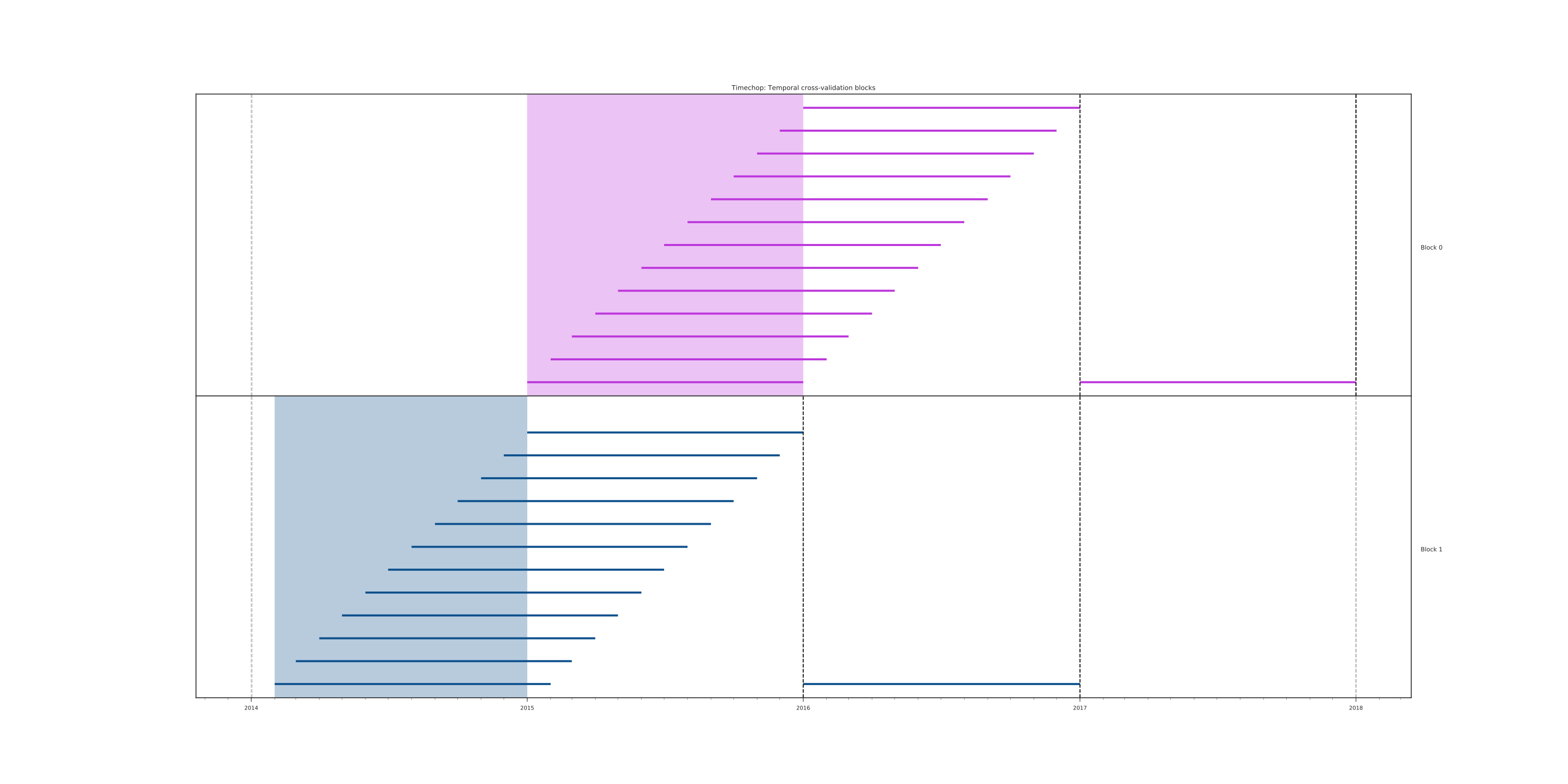

The shaded areas (in this image there is just one per block, but you will see other examples below) represents the span of the as of dates. They start with the oldest as of date and end with the latest. Each line inside that area represents the label span. Those lines begin at the as of date. At each as of date, timechop generates each entity's features (from the past) and labels (from the future). So in the image, we will have two sets of train/test datasets. Each facility will have 13 rows in "Block 0" and 12 rows in "Block 1". The trained models will predict the label using the features calculated for that test set as of date. The single line represents the label's time horizon in testing.

This is the temporal configuration that generated the previous image:
```
temporal_config:
    feature_start_time: '2014-01-01'
    feature_end_time: '2018-01-01'
    label_start_time: '2014-01-02'
    label_end_time: '2018-01-01'

    model_update_frequency: '1y'
    training_label_timespans: ['1y']
    training_as_of_date_frequencies: '1month'

    test_durations: '0d'
    test_label_timespans: ['1y']
    test_as_of_date_frequencies: '1month'

    max_training_histories: '1y'
```
In that configuration the date ranges of features and labels are equal, but they can be different (maybe you have more data for features that data for labels) as is shown in the following image and in their configuration parameters.
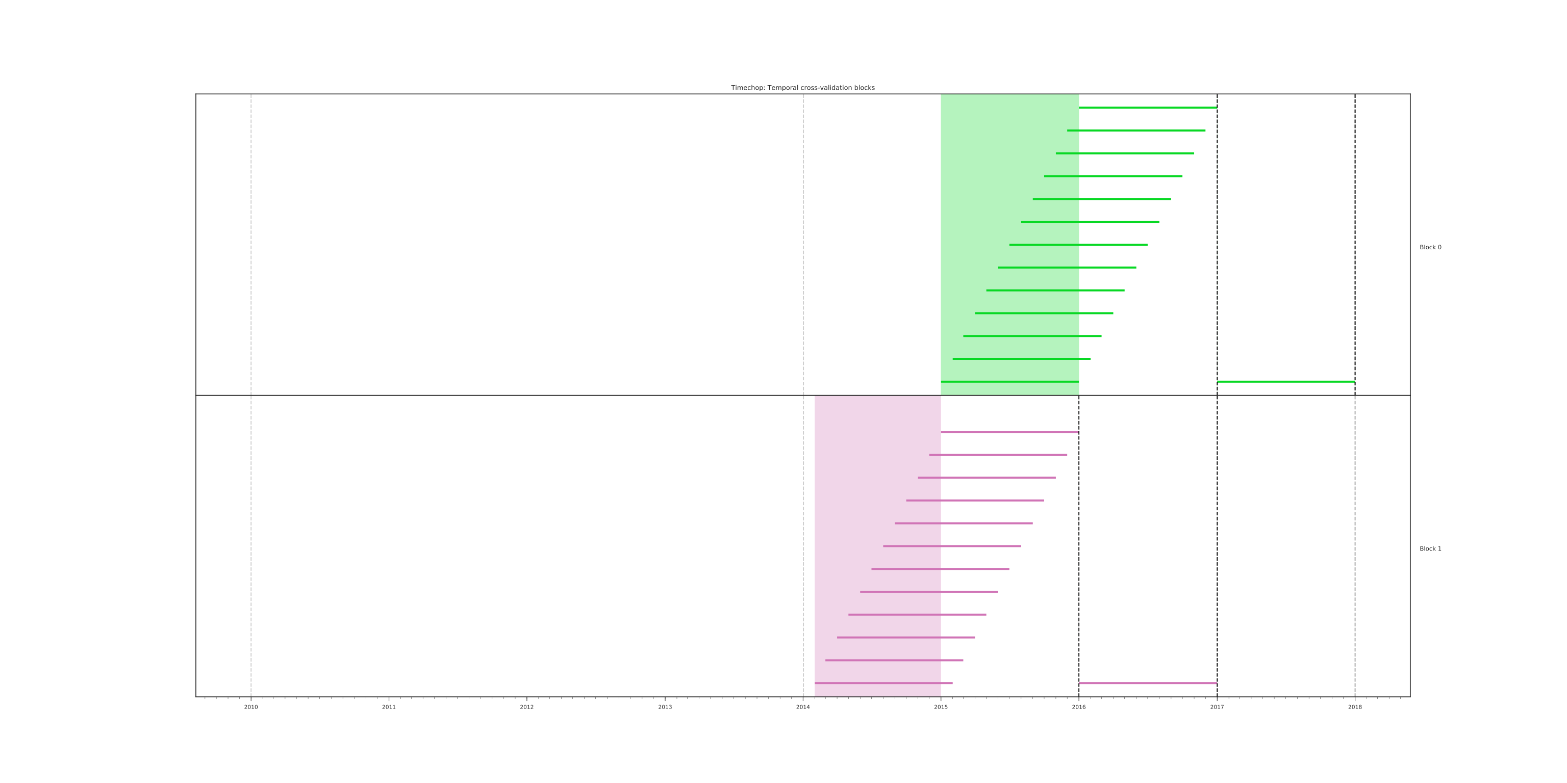
```
temporal_config:
    feature_start_time: '2010-01-01'   # <------- The change happened here!
    feature_end_time: '2018-01-01'
    label_start_time: '2014-01-02'
    label_end_time: '2018-01-01'

    model_update_frequency: '1y'
    training_label_timespans: ['1y']
    training_as_of_date_frequencies: '1month'

    test_durations: '0d'
    test_label_timespans: ['1y']
    test_as_of_date_frequencies: '1month'

    max_training_histories: '1y'
```

model_update_frequency

From our baseline temporal_config example (102), we will change how often we want a new model, which generates more time blocks (if there are time-constrained data, obviously).

temporal_config:
    feature_start_time: '2014-01-01'
    feature_end_time: '2018-01-01'
    label_start_time: '2014-01-02'
    label_end_time: '2018-01-01'

    model_update_frequency: '6month' # <------- The change happened here!
    training_label_timespans: ['1y']
    training_as_of_date_frequencies: '1month'

    test_durations: '0d'
    test_label_timespans: ['1y']
    test_as_of_date_frequencies: '1month'

    max_training_histories: '1y'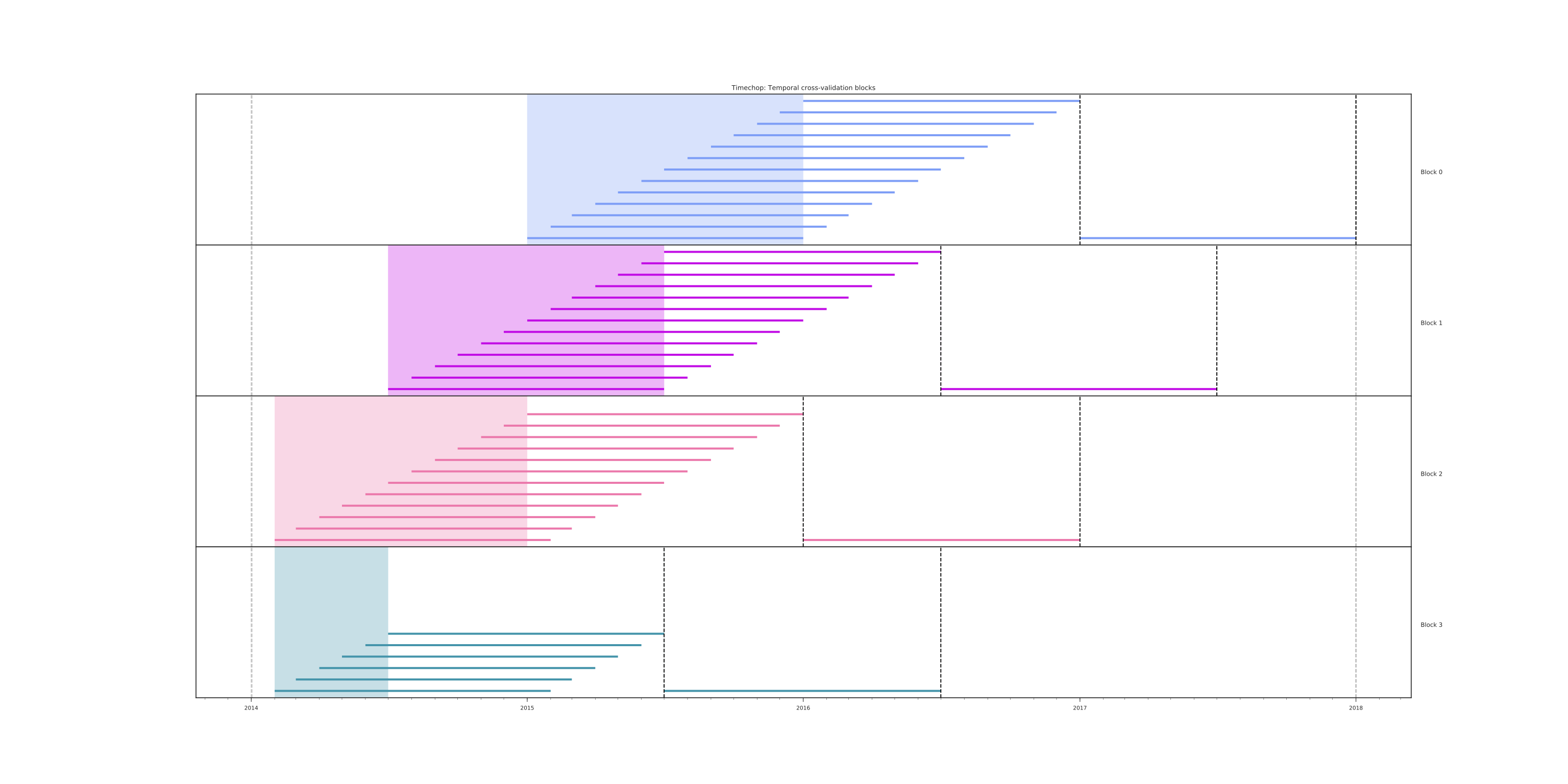

max_training_histories

With this parameter you could get a growing window for training (depicted in 110) or as in all the other examples, fixed training windows.

temporal_config:
    feature_start_time: '2014-01-01'
    feature_end_time: '2018-01-01'
    label_start_time: '2014-01-02'
    label_end_time: '2018-01-01'

    model_update_frequency: '1y'
    training_label_timespans: ['1y']
    training_as_of_date_frequencies: '1month'

    test_durations: '0d'
    test_label_timespans: ['1y']
    test_as_of_date_frequencies: '1month'

    max_training_histories: '10y'  # <------- The change happened here!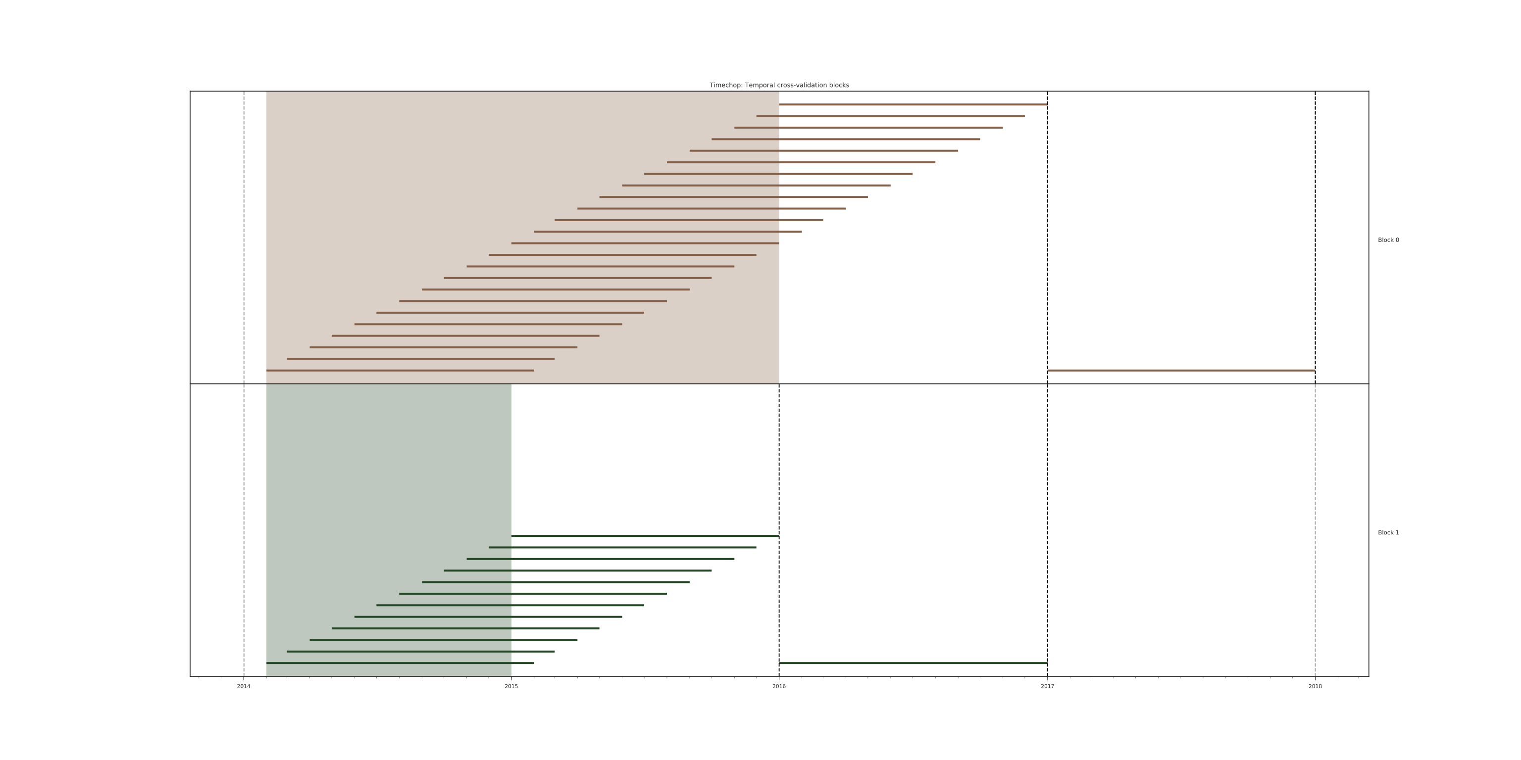

_as_of_date_frequencies and test_durations

temporal_config:
    feature_start_time: '2014-01-01'
    feature_end_time: '2018-01-01'
    label_start_time: '2014-01-02'
    label_end_time: '2018-01-01'

    model_update_frequency: '1y'
    training_label_timespans: ['1y']
    training_as_of_date_frequencies: '3month' # <------- The change happened here!

    test_durations: '0d'
    test_label_timespans: ['1y']
    test_as_of_date_frequencies: '1month'

    max_training_histories: '10y'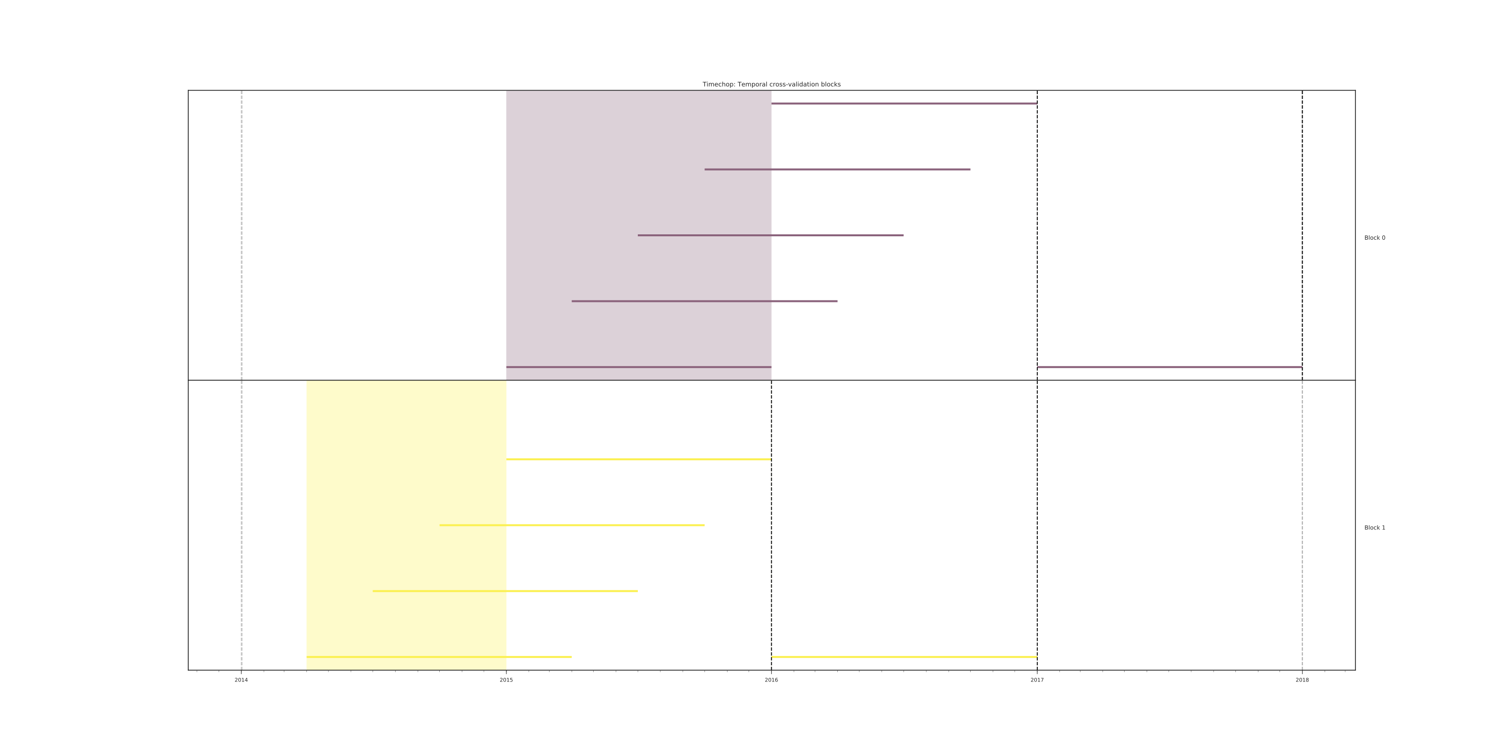

Now, change test_as_of_date_frequencies:

temporal_config:
    feature_start_time: '2014-01-01'
    feature_end_time: '2018-01-01'
    label_start_time: '2014-01-02'
    label_end_time: '2018-01-01'

    model_update_frequency: '1y'
    training_label_timespans: ['1y']
    training_as_of_date_frequencies: '1month'

    test_durations: '0d'
    test_label_timespans: ['1y']
    test_as_of_date_frequencies: '3month'<------- The change happened here!

    max_training_histories: '10y'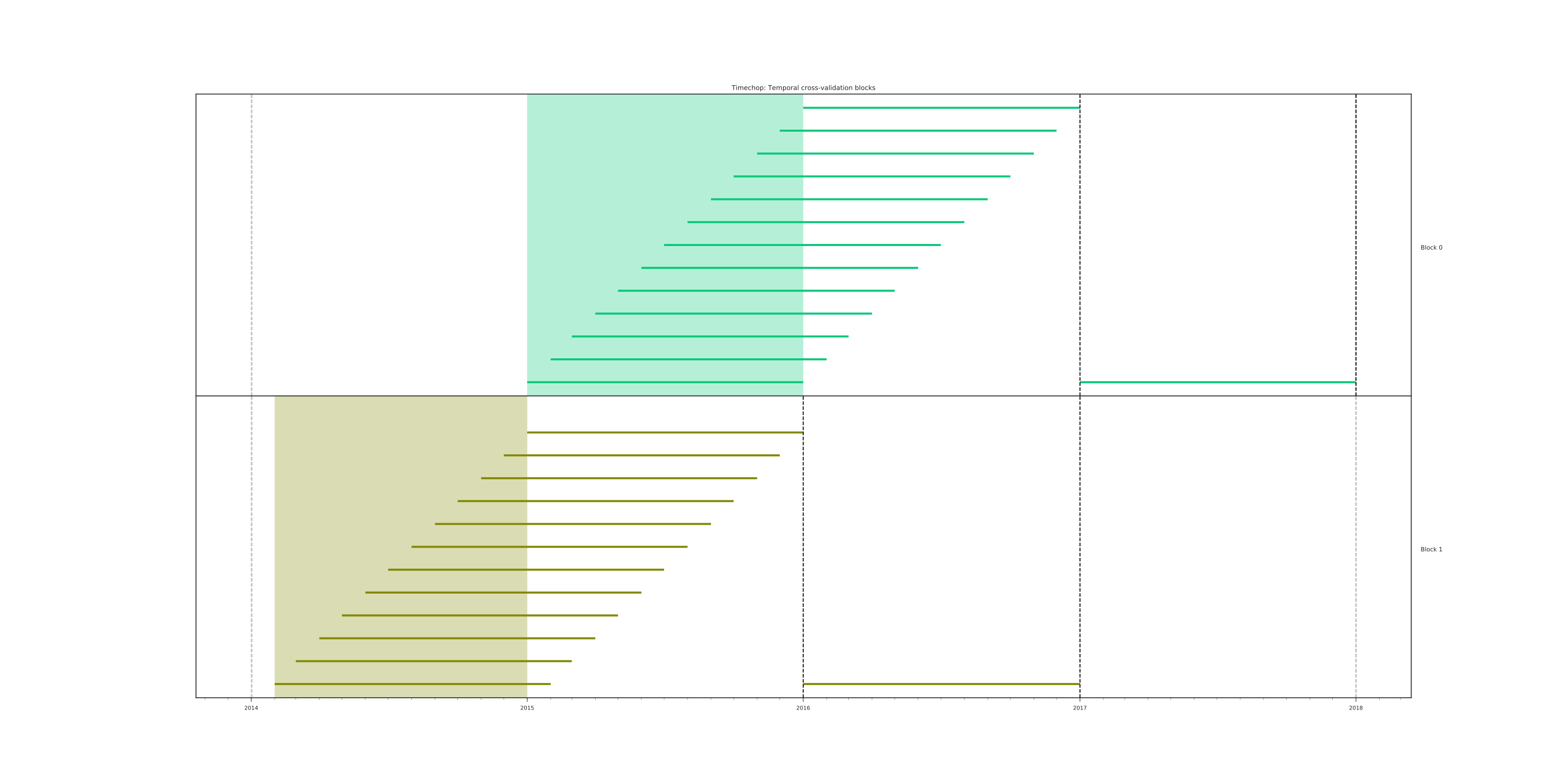

Nothing changed because the test set doesn't have "space" to allow more spans. The "space" is controlled by test_durations, so let's change it to 6month:

temporal_config:
    feature_start_time: '2014-01-01'
    feature_end_time: '2018-01-01'
    label_start_time: '2014-01-02'
    label_end_time: '2018-01-01'

    model_update_frequency: '1y'
    training_label_timespans: ['1y']
    training_as_of_date_frequencies: '1month'

    test_durations: '6month' <------- The change happened here!
    test_label_timespans: ['1y']
    test_as_of_date_frequencies: '1month'

    max_training_histories: '10y'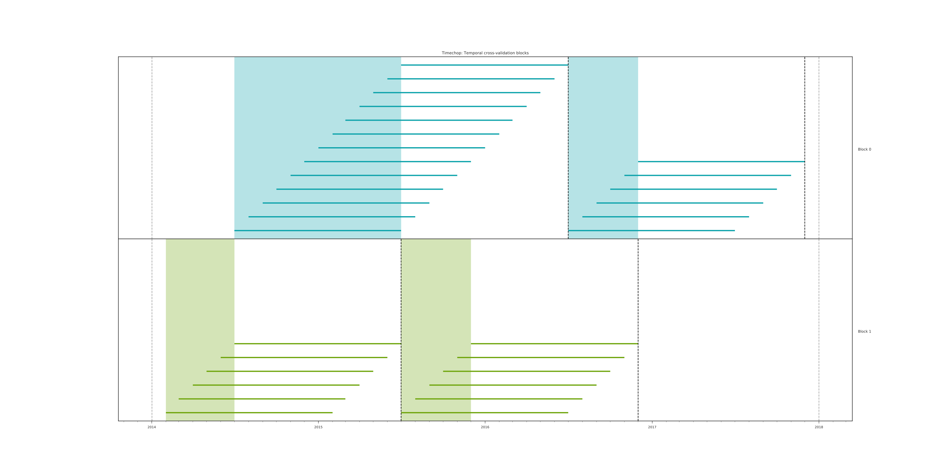

So, now we will move both parameters: test_durations, test_as_of_date_frequencies

temporal_config:
    feature_start_time: '2014-01-01'
    feature_end_time: '2018-01-01'
    label_start_time: '2014-01-02'
    label_end_time: '2018-01-01'

    model_update_frequency: '1y'
    training_label_timespans: ['1y']
    training_as_of_date_frequencies: '1month'

    test_durations: '6month' <------- The change happened here!
    test_label_timespans: ['1y']
    test_as_of_date_frequencies: '3month' <------- and also here!

    max_training_histories: '10y'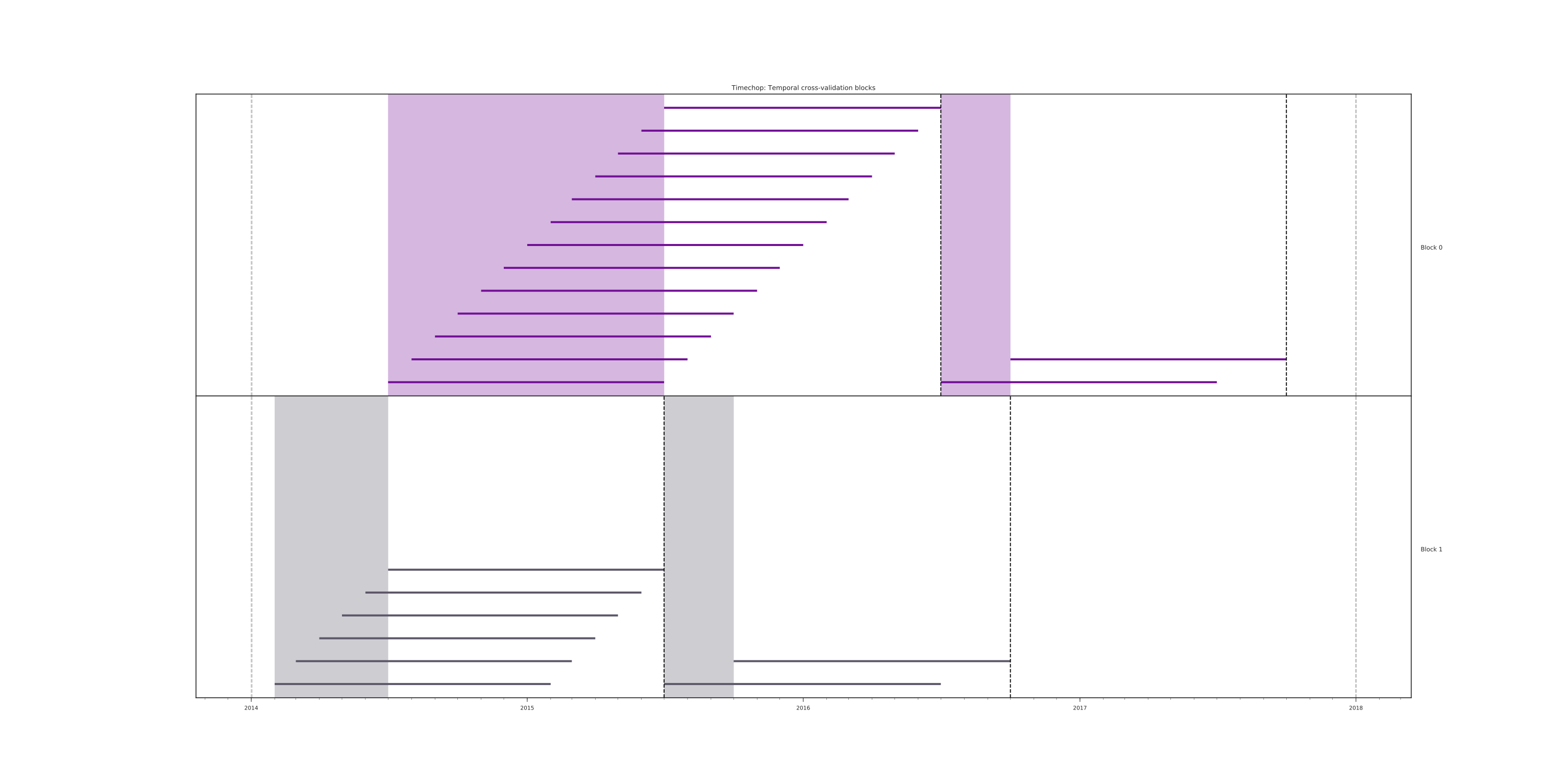

_label_timespans

temporal_config:
    feature_start_time: '2014-01-01'
    feature_end_time: '2018-01-01'
    label_start_time: '2014-01-02'
    label_end_time: '2018-01-01'

    model_update_frequency: '1y'
    training_label_timespans: ['1y']
    training_as_of_date_frequencies: '1month'

    test_durations: '0d'
    test_label_timespans: ['3month']  <------- The change happened here!
    test_as_of_date_frequencies: '1month'

    max_training_histories: '10y'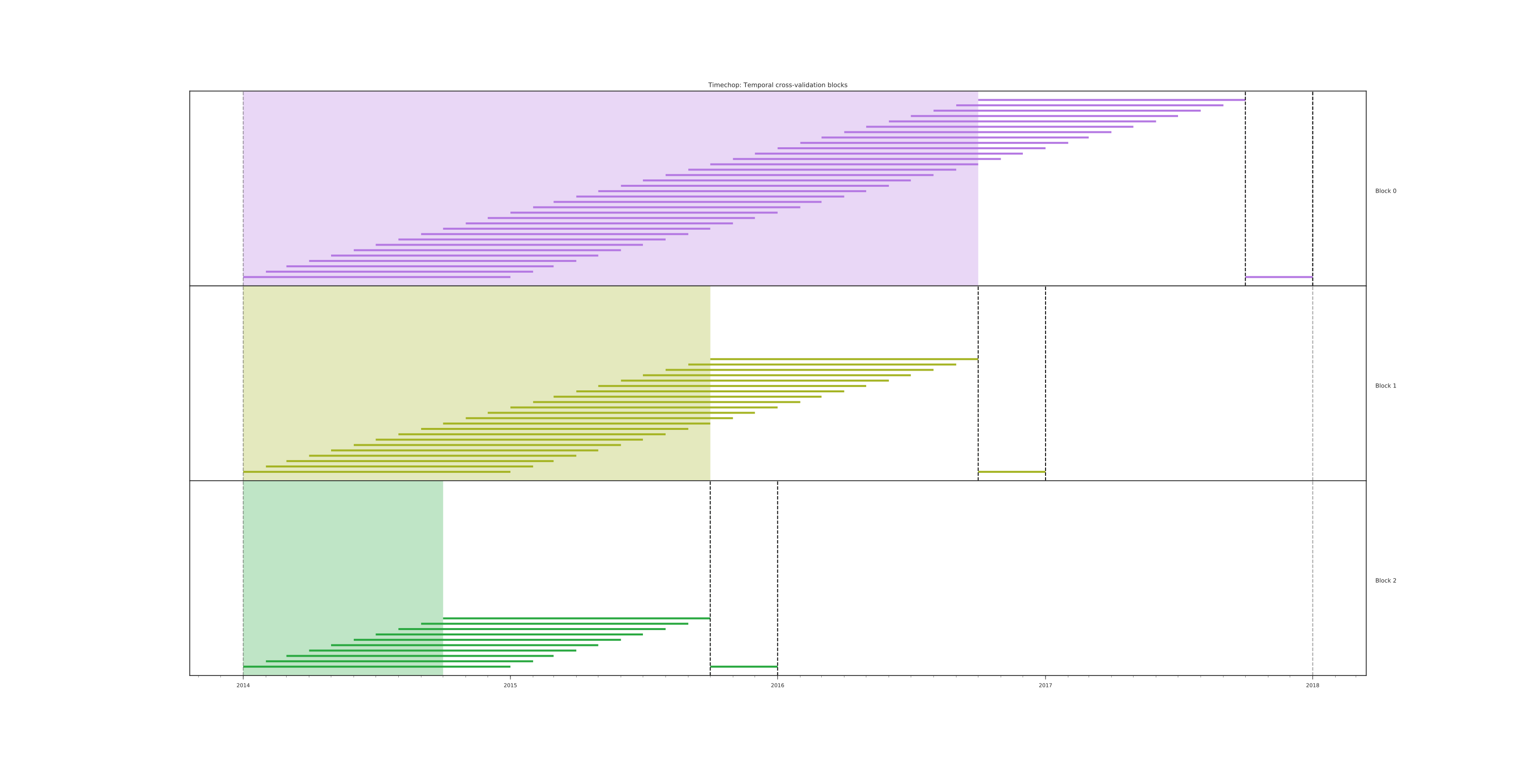

temporal_config:
    feature_start_time: '2014-01-01'
    feature_end_time: '2018-01-01'
    label_start_time: '2014-01-02'
    label_end_time: '2018-01-01'

    model_update_frequency: '1y'
    training_label_timespans: ['3month'] <------- The change happened here!
    training_as_of_date_frequencies: '1month'

    test_durations: '0d'
    test_label_timespans: ['1y']
    test_as_of_date_frequencies: '1month'

    max_training_histories: '10y'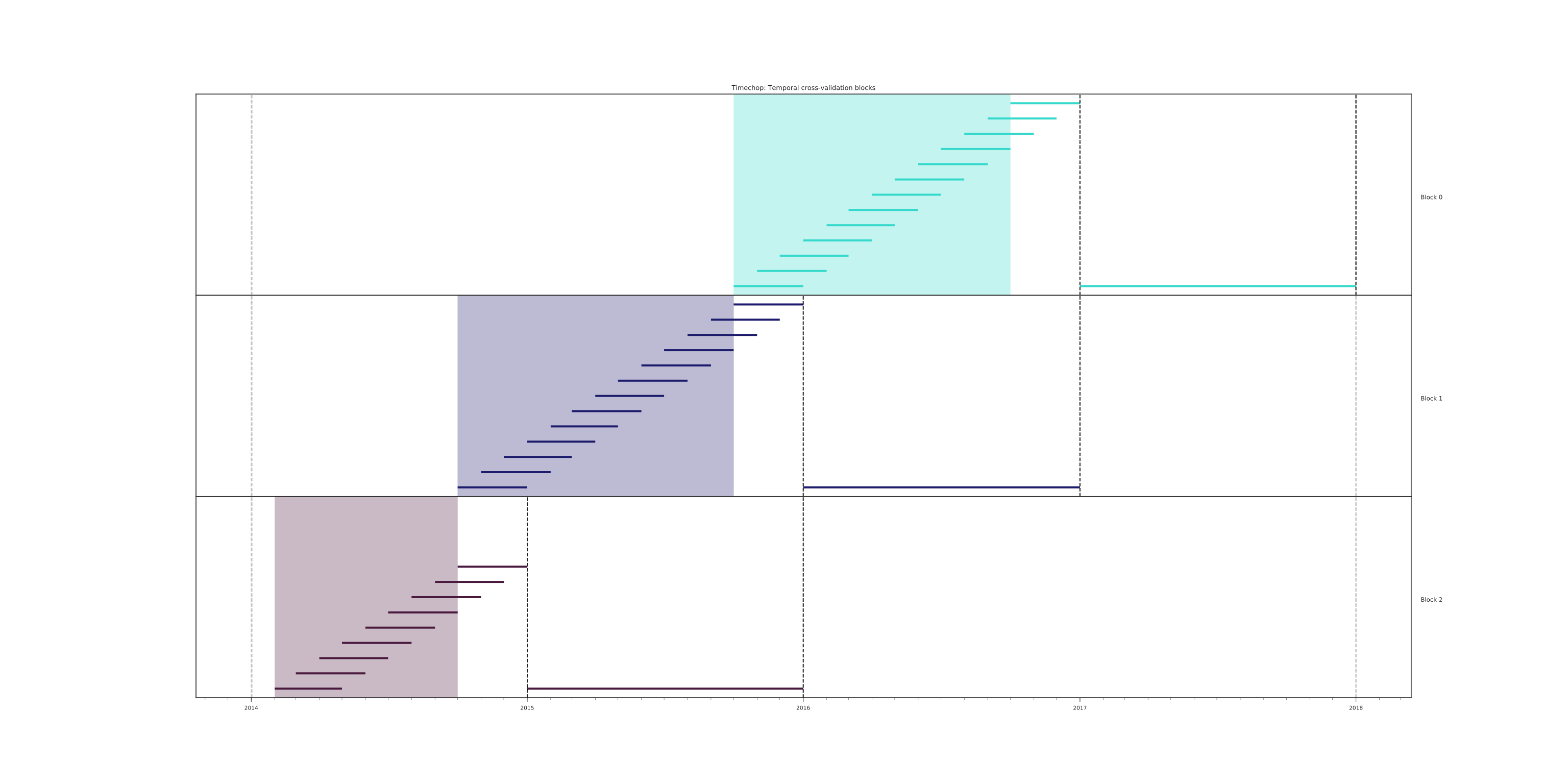

That's it! Now you have the power to bend time!⁸

With the time blocks defined, triage will create the labels and then the features for our train and test sets. We will discuss features in the following section.

Feature generation#

We will show how to create features using the experiments config file. triage uses collate for this.⁹ The collate library controls the generation of features (including the imputation rules for each feature generated) using the time blocks generated by timechop. Collate helps the modeler create features based on spatio-temporal aggregations into the as of date. Collate generates SQL queries that will create features per each as of date.

As before, we will try to mimic what triage does behind the scenario. Collate will help you to create features based on the following template:

For a given as of date, how the aggregation function operates into a column taking into account a previous time interval and some attributes.

Two possible features could be framed as:

As of 2016-01-01, how many inspections
has each facility had in the previous 6 months?

and

As of 2016-01-01, how many "high risk" findings has the
facility had in the previous 6 months?

In our data, that date range (between 2016-01-01 and 2015-07-01) looks like:

select
    event_id,
    date,
    entity_id,
    risk
from
    semantic.events
where
    date <@ daterange(('2016-01-01'::date - interval '6 months')::date, '2016-01-01')
    and entity_id in (229,355,840)
order by
    date asc;

event_id	date	entity_id	risk
1561324	2015-07-17	840	high
1561517	2015-07-24	840	high
1562122	2015-08-12	840	high
1547403	2015-08-20	229	high
1547420	2015-08-28	229	high
1547448	2015-09-14	355	medium
1547462	2015-09-21	355	medium
1547504	2015-10-09	355	medium
1547515	2015-10-16	355	medium
1583249	2015-10-21	840	high
1583577	2015-10-28	840	high
1583932	2015-11-04	840	high

We can transform those data to two features: number_of_inspections and flagged_as_high_risk:

select
    entity_id,
    '2016-01-01' as as_of_date,
    count(event_id) as inspections,
    count(event_id) filter (where risk='high') as flagged_as_high_risk
from
    semantic.events
where
    date <@ daterange(('2016-01-01'::date - interval '6 months')::date, '2016-01-01')
    and entity_id in (229,355,840)
group by
    grouping sets(entity_id);

entity_id	as_of_date	inspections	flagged_as_high_risk
229	2016-01-01	2	2
355	2016-01-01	4	0
840	2016-01-01	6	6

This query is making an aggregation. Note that the previous SQL query has five parts:

The filter ((risk = 'high')::int)
The aggregation function (count())
The name of the resulting transformation (flagged_as_high_risk)
The context in which it is aggregated (by entity_id)
The date range (between 2016-01-01 and 6 months before)

What about if we want to add proportions and totals of failed and passed inspections?

select
    entity_id,
    '2016-01-01' as as_of_date,
    count(event_id) as inspections,
    count(event_id) filter (where risk='high') as flagged_as_high_risk,
    count(event_id) filter (where result='pass') as passed_inspections,
    round(avg((result='pass')::int), 2) as proportion_of_passed_inspections,
    count(event_id) filter (where result='fail') as failed_inspections,
    round(avg((result='fail')::int), 2) as proportion_of_failed_inspections
from
    semantic.events
where
    date <@ daterange(('2016-01-01'::date - interval '6 months')::date, '2016-01-01')
    and entity_id in (229,355,840)
group by
    grouping sets(entity_id)

entity_id	as_of_date	inspections	flagged_as_high_risk	passed_inspections	proportion_of_passed_inspections	failed_inspections	proportion_of_failed_inspections
229	2016-01-01	2	2	1	0.50	1	0.50
355	2016-01-01	4	0	1	0.25	2	0.50
840	2016-01-01	6	6	4	0.67	2	0.33

But what if we want to also add features for "medium" and "low" risk? And what would the query look like if we want to use several time intervals, like 3 months, 5 years, etc? What if we want to contextualize this by location? Plus we need to calculate all these features for several as of dates and manage the imputation strategy for all of them!!!

You will realize that even with this simple set of features we will require very complex SQL to be constructed.

But fear not. triage will automate that for us!

The following blocks of code represent a snippet of triage's configuration file related to feature aggregation. It shows the triage syntax for the inspections feature constructed above:

feature_aggregations:
  -
    prefix: 'inspections'
    from_obj: 'semantic.events'
    knowledge_date_column: 'date'

    aggregates:
      -
        quantity:
          total: "*"
        imputation:
           count:
              type: 'zero_noflag'
        metrics:
          - 'count'

    intervals: ['6month']

feature_aggregations is a yaml list¹⁰ of feature groups construction specification or just feature group. A feature group is a way of grouping several features that share intervals and source data (from_obj). triage requires the following configuration parameter for every feature group:

prefix: This will be used for name of the feature created
from_obj: Represents a TABLE object in PostgreSQL. You can pass a table like in the example above (semantic.events) or a SQL query that returns a table. We will see an example of this later. triage will use it like the FROM clause in the SQL query.
knowlege_date_column: Column that indicates the date of the event.
intervals: A yaml list. triage will create one feature per interval listed.

The last section to discuss is imputation. Imputation is very important step in the modeling, and you should carefully think about how you will impute the missing values in the feature. After deciding the best way of impute each feature, you should avoid leakage (For example, imagine that you want to impute with the mean one feature. You could have leakage if you take all the values of the column, including ones of the future to calculate the imputation). We will return to this later in this tutorial.

Collate is in charge of creating the SQL agregation queries. Another way of thinking about it is that collate encapsulates the FROM part of the query (from_obj) as well as the GROUP BY aggregation at the entity_id level.

triage (collate) supports two types of objects to be aggregated: aggregates and categoricals (more on this one later)¹¹. The aggregates subsection represents a yaml list of features to be created. Each element on this represents a column (quantity, in the example, the whole row *) and an alias (total), defines the imputation strategy for NULLs, and the metric refers to the aggregation function to be applied to the quantity (count).

triage will generate the following (or a very similar one), one per each combination of interval × quantity:

select
  metric(quantity) as alias
from
  from_obj
where
  as_of_date <@ (as_of_date - interval, as_of_date)
group by
  grouping sets(entity_id)

With the previous configuration triage will generate 1 feature with the following name:¹²

inspections_entity_id_6month_total_count

All the features of that feature group (in this case only 1) will be stored in the table.

features.inspections_aggregation_imputed

In general the names of the generated tables are constructed as follows:

schema.prefix_group_aggregation_imputed

NOTE: the outputs are stored in the features schema.

Inside each of those new tables, the feature name will follow this pattern:

prefix_group_interval_alias_aggregation_operation

If we complicate a little the above configuration adding new intervals:

feature_aggregations:
  -
    prefix: 'inspections'
    from_obj: 'semantic.events'
    knowledge_date_column: 'date'

    aggregates:
      - # number of inspections
        quantity:
          total: "*"

        imputation:
          count:
            type: 'zero_noflag'

        metrics: ['count']

    intervals: ['1month', '3month', '6month', '1y', 'all']

You will end with 5 new features, one for each interval (5) × the only aggregate definition we have. Note the weird all in the intervals definition. all is the time interval between the feature_start_time and the as_of_date.

triage also supports categorical objects. The following code adds a feature for the risk flag.

feature_aggregations:
  -
    prefix: 'inspections'
    from_obj: 'semantic.events'
    knowledge_date_column: 'date'

    aggregates:
      - # number of inspections
        quantity:
          total: "*"

        imputation:
          count:
            type: 'zero_noflag'

        metrics: ['count']

    intervals: ['1month', '3month', '6month', '1y', 'all']

  -
    prefix: 'risks'
    from_obj: 'semantic.events'
    knowledge_date_column: 'date'

    categoricals_imputation:
      sum:
        type: 'zero'

    categoricals:
      -
        column: 'risk'
        choice_query: 'select distinct risk from semantic.events'
          metrics:
            - 'sum'

    intervals: ['1month', '3month', '6month', '1y', 'all']

There are several changes. First, the imputation strategy in this new feature group is for every categorical features in that feature group (in that example only one). The next change is the type: instead of aggregates, it's categoricals. categoricals define a yaml list too. Each categorical feature needs to define a column to be aggregated and the query to get all the distinct values.

With this configuration, triage will generate two tables, one per feature group. The new table will be features.risks_aggregation_imputed. This table will have more columns: intervals (5) × metric (1) × features (1) × number of choices returned by the query.

The query:

select distinct risk from semantic.events;

risk
¤
medium
high
low

returns 4 possible values (including NULL). When dealing with categorical aggregations you need to be careful. Could be the case that in some period of time, in your data, you don't have all the possible values of the categorical variable. This could cause problems down the road. Triage allows you to specify the possible values (choices) of the variable. Instead of using choice_query, you could use choices as follows:

feature_aggregations:
  -
    prefix: 'inspections'
    from_obj: 'semantic.events'
    knowledge_date_column: 'date'

    aggregates:
      - # number of inspections
        quantity:
          total: "*"

        imputation:
          count:
            type: 'mean'

        metrics: ['count']

    intervals: ['1month', '3month', '6month', '1y', 'all']

  -
    prefix: 'risks'
    from_obj: 'semantic.events'
    knowledge_date_column: 'date'

    categoricals_imputation:
      sum:
        type: 'zero'

    categoricals:
      -
        column: 'risk'
        choices: ['low', 'medium', 'high']
          metrics:
            - 'sum'

    intervals: ['1month', '3month', '6month', '1y', 'all']

In both cases triage will generate 20 new features, as expected.

The features generated from categorical objects will have the following pattern:

prefix_group_interval_column_choice_aggregation_operation

So, risks_entity_id_1month_risk_medium_sum will be among our new features in the last example.

Triage will also add several imputation flag (binary) columns per feature. Those columns convey information about if that particular value was imputed or not. The section below describes how imputation can be specified in triage in more detail.

Imputation#

Triage currently supports the following imputation strategies:

mean: The mean value of the feature.
constant: Fill with a constant (you need to provide the constant value).
zero: Same that the previous one, but the constant is zero.
zero_noflag: Sometimes, the absence (i.e. a NULL) doesn't mean that the value is missing, that actually means that the event didn't happen to that entity. For example a NULL in the inspections_entity_id_1month_total_count column in features.inspections_aggreagtion_imputed doesn't mean that the value is missing, it means that zero inspections happen to that facility in the last month. Henceforth, the flag column is not needed.

Only for aggregates:

binary_mode: Takes the mode of a binary feature

Only for categoricals:

null_category: Just flag null values with the null category column

and finally, if you are sure that is not possible to have NULLS:

error: Raise an exception if ant null values are encountered.

Feature groups strategies#

Another interesting thing that triage controls is how many feature groups are used in the machine learning grid. This would help you to understand the effect of using different groups in the final performance of the models.

In simple_test_skeleton.yaml you will find the following blocks:

feature_group_definition:
  prefix:
    - 'results'
    - 'risks'
    - 'inspections'

feature_group_strategies: ['all']

This configuration adds to the number of model groups to be created.

The possible feature group strategies are:

all: All the features groups are used.
leave-one-out: All the combinations of: "All the feature groups except one are used".
leave-one-in: All the combinations of "One feature group except the rest is used"
all-combinations: All the combinations of feature groups

In order to clarify these concepts, let's use simple_test_skeleton.yaml configuration file. In it there are three feature groups: inspections, results, risks.

Using all will create just one set containg all the features of the three feature groups:

{inspections, results, risks}

If you modify feature_group_strategies to ['leave-one-out']: the following sets will be created:

{inspections, results}, {inspections, risks}, {results, risks}

Using the leave-one-in strategy:

{inspections}, {results}, {risks}

Finally choosing all-combinations:

{inspections}, {results}, {risks}, {inspections, results}, {inspections, risks}, {results, risks}, {inspections, results, risks}

Controlling the size of the tables#

This section is a little technical, you can skip it if you fell like it.

By default, triage will use the biggest column type for the features table (integer, numeric, etc). This could lead to humongous tables, with sizes several hundred of gigabytes. Triage took that decision, because it doesn't know anything about the possible values of your data (e.g. Is it possible to have millions of inspections in one month? or just a few dozens?).

If you are facing this difficulty, you can force triage to cast the column in the features table. Just add coltype to the aggregate/categorical block:

 aggregates:
   -
    quantity:
      total: "*"
    metrics: ['count']
    coltype: 'smallint'

The Grid#

Before applying Machine Learning to your dataset you don't know which combination of algorithm and hyperparameters will be the best given a specific matrix.

Triage approaches this problem exploring a algorithm + hyperparameters + feature groups grid. At this time, this exploration is a exhaustive one, i.e. it covers the complete grid, so you would get (number of algorithms) $\times$ (number of hyperparameters) $\times$ (number of feature group strategies) models groups. The number of models trained is (number of model groups) $\times$ (number of time splits).

In our simple experiment the grid is very simple:

grid_config:
    'sklearn.dummy.DummyClassifier':
        strategy: [most_frequent]

Just one algorithm and one hyperparameter (also we have only one feature group strategy: all), and two time splits. So we will get 2 models, 1 model group.

Keep in mind that the grid is providing more than way to select a model. You can use the tables generated by the grid (see section Machine Learning Governance ) and analyze and understand your data. In other words, analyzing the results (evaluations, predictions, hyperparameter space, etc.) is like applying Data mining concepts to your data using Machine learning. We will return to this when we apply post modeling to our models.

Audition#

Audition is a tool for helping you select a subset of trained classifiers from a triage experiment. Often, production-scale experiments will come up with thousands of trained models, and sifting through all of those results can be time-consuming even after calculating the usual basic metrics like precision and recall.

You will be facing questions as:

Which metrics matter most?
Should you prioritize the best metric value over time or treat recent data as most important?
Is low metric variance important?

The answers to questions like these may not be obvious. Audition introduces a structured, semi-automated way of filtering models based on what you consider important.

Post-modeling#

As the name indicates, postmodeling occurs after you have modeled (potentially) thousands of models (different hyperparameters, different time windows, different algorithms, etc), and using audition you pre selected a small number of models.

Now, with the postmodeling tools you will be able to select your final model for production use.

Triage's postmodeling capabilities include:

Show the score distribution
Compare the list generated by a set of models
Compare the feature importance between a set of models
Diplay the probability calibration curves
Analyze the errors using a decision tree trained on the errors of the model.
Cross-tab analysis
Bias analysis

If you want to see Audition and Postmodeling in action, we will use them after Inspections and EIS modeling.

Final cleaning#

In the next section we will start modeling, so it is a good idea to clean the {test, train}_results schemas and have a fresh start:

select nuke_triage();

nuke_triage
triage was send to the oblivion. Long live to triage!

triage also creates a lot of files (we will see why in the next section). Let's remove them too.

rm -r /triage/matrices/*

rm -r /triage/trained_models/*

Where to go from here...#

If you haven't done so already, our dirty duck tutorial is a good way to geet up and running with some sample data.

If you're ready to get started with your own data, check out the suggested project workflow for some tips about how to iterate and tune the pipeline for your project.

Footnotes#

¹ Would be my restaurant inspected in the following month? in the case of an early warning case.

² It's a little more complicated than that as we will see.

³ All events produce some outcome. In theory every event of interest in stored in a database. These events are immutable: you can't (shouldn't) change them (they already happen).

⁴ We could consider different states, for example: we can use the column risk as an state. Another possibility is define a new state called failed that indicates if the facility failed in the last time it was inspected. One more: you could create cohorts based on the facility_type.

⁵ The city in this toy example has very low resources.

⁶ See for example: https://robjhyndman.com/hyndsight/tscv/

⁷ I know, I know. And in order to cover all the cases, we are still missing one or two parameters, but we are working on it.

⁸ Obscure reference to the "Avatar: The Last Airbender" cartoon series. I'm sorry.

⁹ collate is to feature generation what timechop is to date temporal splitting

¹⁰ triage uses a lot of yaml, this guide could be handy

¹¹ Note that the name categoricals is confusing here: The original variable (i.e. a column) is categorical, the aggregate of that column is not. The same with the aggregates: The original column could be a categorical or a numeric (to be fare most of the time is a numeric column, but see the example: we are counting), and then triage applies an aggregate that will be numeric. That is how triage named things, and yes, I know is confusing.

¹² triage will generate also a new binary column that indicates if the value of the feature was imputed (1) or not (0): inspections_entity_id_6month_total_count_imp.