COMPAS Analysis using Aequitas

Recent work in the Machine Learning community has raised concerns about the risk of unintended bias in Algorithmic Decision-Making systems, affecting individuals unfairly. While many bias metrics and fairness definitions have been proposed in recent years, the community has not reached a consensus on which definitions and metrics should be used, and there has been very little empirical analyses of real-world problems using the proposed metrics.

We present the Aequitas toolkit as an intuitive addition to the machine learning workflow, enabling users to to seamlessly test models for several bias and fairness metrics in relation to multiple population groups. We believe the tool will faciliate informed and equitable decision-making around developing and deploying predictive risk-assessment tools for both machine learnining practitioners and policymakers, allowing researchers and program managers to answer a host of questions related to machine learning models, including:

• What biases exist in my model?

  • What is the distribution of groups, predicted scores, and labels across my dataset?

  • What are bias metrics across groups?

  • How do I interpret biases in my model?

  • How do I visualize biases in my model?

• What levels of disparity exist between population groups?

  • How does the selected reference group affect disparity calculations?

  • How do I interpret calculated disparity ratios?

  • How do I visualize disparities in my model?

• How do I assess model fairness??

  • How do I interpret parities?

  • How do I visualize bias metric parity?

  • How do I visualize parity between groups in my model?

We apply the toolkit to the COMPAS dataset reported on by ProPublica below.

Background

In 2016, ProPublica reported on racial inequality in automated criminal risk assessment algorithms. The report is based on this analysis. Using a clean version of the COMPAS dataset from the ProPublica GitHub repo, we demostrate the use of the Aequitas bias reporting tool.

Northpointe’s COMPAS (Correctional Offender Management Profiling for Alternative Sanctions) is one of the most widesly utilized risk assessment tools/ algorithms within the criminal justice system for guiding decisions such as how to set bail. The ProPublica dataset represents two years of COMPAS predicitons from Broward County, FL.

import pandas as pd
import seaborn as sns
from aequitas.group import Group
from aequitas.bias import Bias
from aequitas.fairness import Fairness
from aequitas.plotting import Plot

import warnings; warnings.simplefilter('ignore')

%matplotlib inline

/Users/lorenh/Documents/DSaPP/.aequitas/lib/python3.6/importlib/_bootstrap.py:219: RuntimeWarning: numpy.dtype size changed, may indicate binary incompatibility. Expected 96, got 88
  return f(*args, **kwds)

df = pd.read_csv("../../../examples/data/compas_for_aequitas.csv")
df.head()

	entity_id	score	label_value	race	sex	age_cat
0	1	0.0	0	Other	Male	Greater than 45
1	3	0.0	1	African-American	Male	25 - 45
2	4	0.0	1	African-American	Male	Less than 25
3	5	1.0	0	African-American	Male	Less than 25
4	6	0.0	0	Other	Male	25 - 45

df.shape

(7214, 6)

Pre-Aequitas: Exploring the COMPAS Dataset

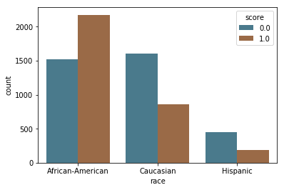
Risk assessment by race

COMPAS produces a risk score that predicts a person’s likelihood of commiting a crime in the next two years. The output is a score between 1 and 10 that maps to low, medium or high. For Aequitas, we collapse this to a binary prediction. A score of 0 indicates a prediction of “low” risk according to COMPAS, while a 1 indicates “high” or “medium” risk.

This categorization is based on ProPublica’s interpretation of Northpointe’s practioner guide:

"According to Northpointe’s practitioners guide, COMPAS “scores in the medium and high range
garner more interest from supervision agencies than low scores, as a low score would suggest
there is little risk of general recidivism,” so we considered scores any higher than “low” to
indicate a risk of recidivism."

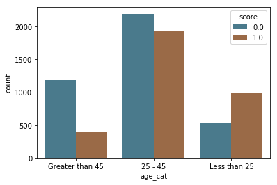
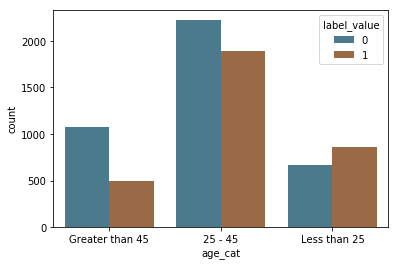
In the bar charts below, we see a large difference in how these scores are distributed by race, with a majority of white and Hispanic people predicted as low risk (score = 0) and a majority of black people predicted high and medium risk (score = 1). We also see that while the majority of people in age categories over 25 are predicted as low risk (score = 0), the majority of people below 25 are predicted as high and medium risk (score = 1).

aq_palette = sns.diverging_palette(225, 35, n=2)

by_race = sns.countplot(x="race", hue="score", data=df[df.race.isin(['African-American', 'Caucasian', 'Hispanic'])], palette=aq_palette)

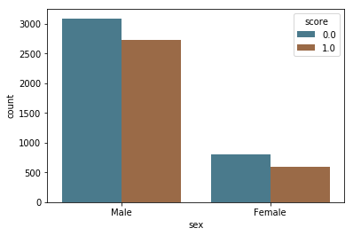
by_sex = sns.countplot(x="sex", hue="score", data=df, palette=aq_palette)

by_age = sns.countplot(x="age_cat", hue="score", data=df, palette=aq_palette)

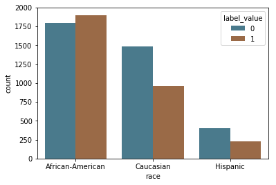
Levels of recidivism

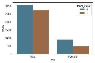
This dataset includes information about whether or not the subject recidivated, and so we can directly test the accuracy of the predictions. First, we visualize the recidivsm rates across race.

Following ProPublica, we defined recidivism as a new arrest within two years. (If a person recidivates, label_value = 1). They “based this decision on Northpointe’s practitioners guide, which says that its recidivism score is meant to predict ‘a new misdemeanor or felony offense within two years of the COMPAS administration date.’”

label_by_race = sns.countplot(x="race", hue="label_value", data=df[df.race.isin(['African-American', 'Caucasian', 'Hispanic'])], palette=aq_palette)

label_by_age = sns.countplot(x="sex", hue="label_value", data=df, palette=aq_palette)

label_by_sex = sns.countplot(x="age_cat", hue="label_value", data=df, palette=aq_palette)

Putting Aequitas to the task

The graphs above show the base rates for recidivism are higher for black defendants compared to white defendants (.51 vs .39), though the predictions do not match the base rates.

Practitioners face the challenge of determining whether or not such patterns reflect bias or not. The fact that there are multiple ways to measure bias adds complexity to the decision-making process. With Aequitas, we provide a tool that automates the reporting of various fairness metrics to aid in this process.

Applying Aequitas progammatically is a three step process represented by three python classes:

Group(): Define groups

Bias(): Calculate disparities

Fairness(): Assert fairness

Each class builds on the previous one expanding the output DataFrame.

Data Formatting

Data for this example was preprocessed for compatibility with Aequitas. The Aequitas tool always requires a ``score`` column and requires a binary ``label_value`` column for supervised metrics, (i.e., False Discovery Rate, False Positive Rate, False Omission Rate, and False Negative Rate).

Preprocessing includes but is not limited to checking for mandatory score and label_value columns as well as at least one column representing attributes specific to the data set. See documentation for more information about input data.

Note that while entity_id is not necessary for this example, Aequitas recognizes entity_id as a reserve column name and will not recognize it as an attribute column.

Back to Top

What biases exist in my model?

Aequitas Group() Class

What is the distribution of groups, predicted scores, and labels across my dataset?

Aequitas’s Group() class enables researchers to evaluate biases across all subgroups in their dataset by assembling a confusion matrix of each subgroup, calculating commonly used metrics such as false positive rate and false omission rate, as well as counts by group and group prevelance among the sample population.

The ``get_crosstabs()`` method tabulates a confusion matrix for each subgroup and calculates commonly used metrics such as false positive rate and false omission rate. It also provides counts by group and group prevelances.

Group Counts Calculated:

Count Type	Column Name
False Positive Count	‘fp’
False Negative Count	‘fn’
True Negative Count	‘tn’
True Positive Count	‘tp’
Predicted Positive Count	‘pp’
Predicted Negative Count	‘pn’
Count of Negative Labels in Group	‘group_label_neg’
Count of Positive Labels in Group	‘group_label_pos’
Group Size	‘group_size’
Total Entities	‘total_entities’

Absolute Metrics Calculated:

Metric	Column Name
True Positive Rate	‘tpr’
True Negative Rate	‘tnr’
False Omission Rate	‘for’
False Discovery Rate	‘fdr’
False Positive Rate	‘fpr’
False Negative Rate	‘fnr’
Negative Predictive Value	‘npv’
Precision	‘precision’
Predicted Positive Ratio	‘ppr’
Predicted Positive Ratio	‘pprev’
Group Prevalence	‘prev’

Note: The ``get_crosstabs()`` method expects a dataframe with predefined columns score, and label_value and treats other columns (with a few exceptions) as attributes against which to test for disparities. In this case, we include race, sex and age_cat.

g = Group()
xtab, _ = g.get_crosstabs(df)

model_id, score_thresholds 1 {'rank_abs': [3317]}
COUNTS::: race
African-American    3696
Asian                 32
Caucasian           2454
Hispanic             637
Native American       18
Other                377
dtype: int64
COUNTS::: sex
Female    1395
Male      5819
dtype: int64
COUNTS::: age_cat
25 - 45            4109
Greater than 45    1576
Less than 25       1529
dtype: int64

Back to Top

What are bias metrics across groups?

Once you have run the Group() class ``get_crosstabs()`` method, you’ll have a dataframe of the group counts and group value bias metrics.

The Group() class has a ``list_absolute_metrics()`` method, which you can use for faster slicing to view just counts or bias metrics.

absolute_metrics = g.list_absolute_metrics(xtab)

View calculated counts across sample population groups

xtab[[col for col in xtab.columns if col not in absolute_metrics]]

	attribute_name	attribute_value	k	model_id	score_threshold	pp	pn	fp	fn	tn	tp	group_label_neg	group_label_pos	group_size	total_entities
0	race	African-American	3317	1	binary 0/1	2174	1522	805	532	990	1369	1795	1901	3696	7214
1	race	Asian	3317	1	binary 0/1	8	24	2	3	21	6	23	9	32	7214
2	race	Caucasian	3317	1	binary 0/1	854	1600	349	461	1139	505	1488	966	2454	7214
3	race	Hispanic	3317	1	binary 0/1	190	447	87	129	318	103	405	232	637	7214
4	race	Native American	3317	1	binary 0/1	12	6	3	1	5	9	8	10	18	7214
5	race	Other	3317	1	binary 0/1	79	298	36	90	208	43	244	133	377	7214
6	sex	Female	3317	1	binary 0/1	591	804	288	195	609	303	897	498	1395	7214
7	sex	Male	3317	1	binary 0/1	2726	3093	994	1021	2072	1732	3066	2753	5819	7214
8	age_cat	25 - 45	3317	1	binary 0/1	1924	2185	741	706	1479	1183	2220	1889	4109	7214
9	age_cat	Greater than 45	3317	1	binary 0/1	394	1182	181	285	897	213	1078	498	1576	7214
10	age_cat	Less than 25	3317	1	binary 0/1	999	530	360	225	305	639	665	864	1529	7214

View calculated absolute metrics for each sample population group

xtab[['attribute_name', 'attribute_value'] + absolute_metrics].round(2)

	attribute_name	attribute_value	tpr	tnr	for	fdr	fpr	fnr	npv	precision	ppr	pprev	prev
0	race	African-American	0.72	0.55	0.35	0.37	0.45	0.28	0.65	0.63	0.66	0.59	0.51
1	race	Asian	0.67	0.91	0.12	0.25	0.09	0.33	0.88	0.75	0.00	0.25	0.28
2	race	Caucasian	0.52	0.77	0.29	0.41	0.23	0.48	0.71	0.59	0.26	0.35	0.39
3	race	Hispanic	0.44	0.79	0.29	0.46	0.21	0.56	0.71	0.54	0.06	0.30	0.36
4	race	Native American	0.90	0.62	0.17	0.25	0.38	0.10	0.83	0.75	0.00	0.67	0.56
5	race	Other	0.32	0.85	0.30	0.46	0.15	0.68	0.70	0.54	0.02	0.21	0.35
6	sex	Female	0.61	0.68	0.24	0.49	0.32	0.39	0.76	0.51	0.18	0.42	0.36
7	sex	Male	0.63	0.68	0.33	0.36	0.32	0.37	0.67	0.64	0.82	0.47	0.47
8	age_cat	25 - 45	0.63	0.67	0.32	0.39	0.33	0.37	0.68	0.61	0.58	0.47	0.46
9	age_cat	Greater than 45	0.43	0.83	0.24	0.46	0.17	0.57	0.76	0.54	0.12	0.25	0.32
10	age_cat	Less than 25	0.74	0.46	0.42	0.36	0.54	0.26	0.58	0.64	0.30	0.65	0.57

Back to Top

How do I interpret biases in my model?

In the slice of the crosstab dataframe created by the Group() class ``get_crosstabs()`` method directly above, we see that African-Americans have a false positive rate (fpr) of 45%, while Caucasians have a false positive rate of only 23%. This means that African-American people are far more likely to be falsely labeled as high-risk than white people. On the other hand, false ommision rates (for) and false discovery rates (fdr) are much closer for those two groups.

Back to Top

How do I visualize bias in my model?

Absolute group bias metrics metrics from the crosstab dataframe created by the Group() class ``get_crosstabs()`` can be visualized with two methods in the Aequitas Plot() class.

One metric can be specified with ``plot_group_metric()``, or a list of particular metrics of interest (or 'all' metrics) can be plotted with ``plot_group_metric_all()``.

aqp = Plot()

Visualizing a single absolute group metric across all population groups

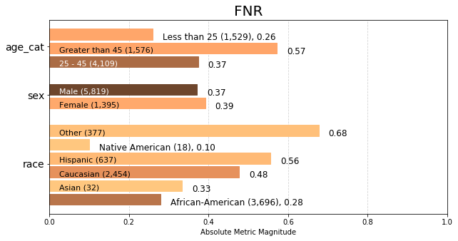
The chart below displays group metric False Negative Rate (fnr) calculated across each attribute, colored based on number of samples in the attribute group.

We can see from the longer bars that across ‘age_cat’, ‘sex’, and ‘race’ attributes, the groups COMPAS incorrectly predicts as ‘low’ or ‘medium’ risk most often are 25-45, Male, and African American. From the darker coloring, we can also tell that these are the three largest populations in the data set.

fnr = aqp.plot_group_metric(xtab, 'fnr')

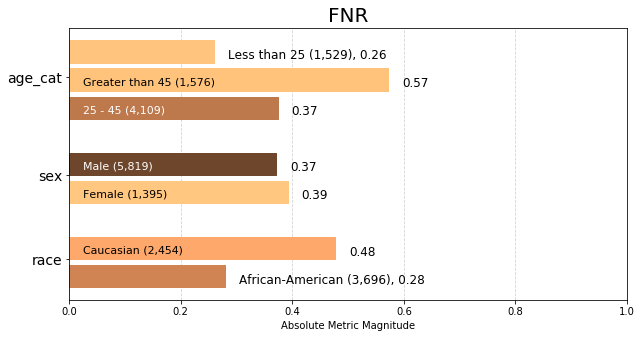
View group metrics for only groups over a certain size threshold

Extremely small group sizes increase standard error of estimates, and could be factors in prediction error such as false negatives. Use the min_group parameter to vizualize only those sample population groups above a user-specified percentage of the total sample size. When we remove groups below 5% of the sample size, we are left with only two of the six ‘race’ groups, as there are much smaller groups in that attribute category than in ‘sex’ or ‘age_cat’ (age cateogry).

fnr = aqp.plot_group_metric(xtab, 'fnr', min_group_size=0.05)

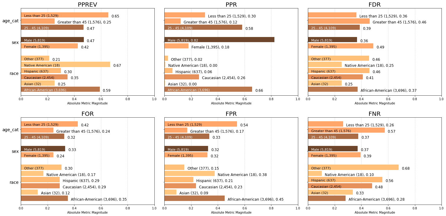
Visualizing multiple user-specified absolute group metrics across all population groups

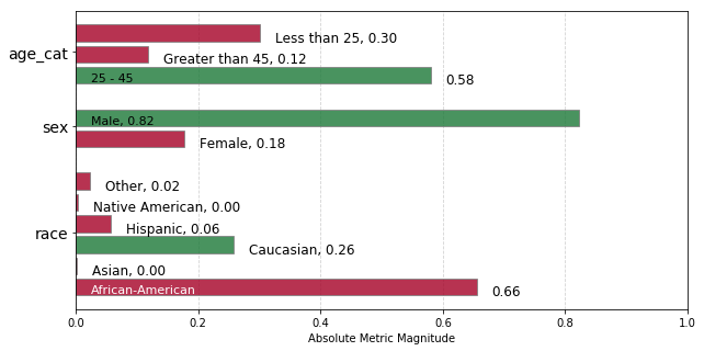
The charts below display the all calculated group metrics across each attribute, colored based on absolute metric magnitude.

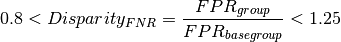
We can see that the largest ‘race’ group, African Americans, are predicted positive more often than any other race group (predicted positive rate PPR of 0.66), and are more likely to be incorrectly classified as ‘high’ risk (false positive rate FPR of 0.45) than incorrectly classified as ‘low’ or ‘medium’ risk (false negative rate FNR of 0.28). Note that Native Americans are predicted positive at a higher prevalence PPREVin relation to their group size than all other ‘race groups’ (predicted prevalence of 0.67).

p = aqp.plot_group_metric_all(xtab, metrics=['ppr','pprev','fnr','fpr'], ncols=4)

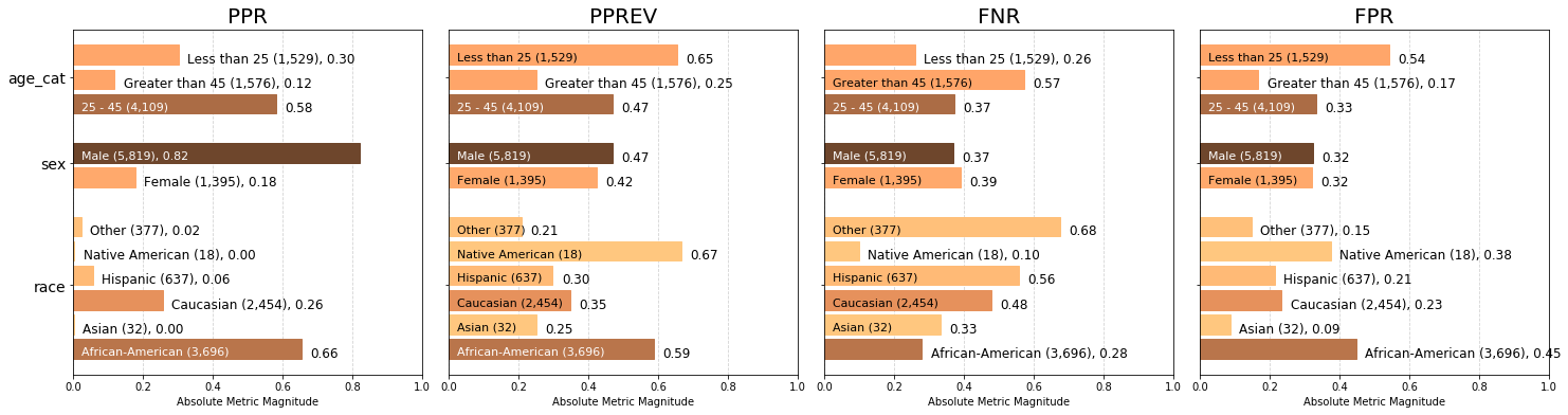
Visualizing default absolute group metrics across all population groups

Default absolute group metrics

When visualizing more than one absolute group metric, you can specify a list of metrics, specify 'all' metrics, or use the Aequitas default metrics by not supplying an argument: - Predicted Positive Group Rate Disparity (pprev), - Predicted Positive Rate Disparity (ppr),

- False Discovery Rate (fdr), - False Omission Rate (for) - False Positive Rate (fpr) - False Negative Rate (fnr)

The charts below display the default group metrics calculated across each attribute, colored based on number of samples in the attribute group.

Note that the 45+ age category is almost twice as likely to be incorrectly included in an intervention group (false discovery rate FDR of 0.46) than incorrectly excluded from intervention (false omission rate FOR 0.24). We can also see that the model is equally likely to predict a woman as ‘high’ risk as it is for a man (false positive rate FPR of 0.32 for both Male and Female).

a = aqp.plot_group_metric_all(xtab, ncols=3)

Back to Top

What levels of disparity exist between population groups?

Aequitas Bias() Class

We use the Aequitas Bias() class to calculate disparities between groups based on the crosstab returned by the Group() class ``get_crosstabs()`` method described above. Disparities are calculated as a ratio of a metric for a group of interest compared to a base group. For example, the False Negative Rate Disparity for black defendants vis-a-vis whites is:

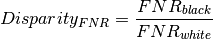
Below, we use ``get_disparity_predefined_groups()`` which allows us to choose reference groups that clarify the output for the practitioner.

The Aequitas Bias() class includes two additional get disparity functions: ``get_disparity_major_group()`` and ``get_disparity_min_metric()``, which automate base group selection based on sample majority (across each attribute) and minimum value for each calculated bias metric, respectively.

The ``get_disparity_predefined_groups()`` allows user to define a base group for each attribute, as illustrated below.

Disparities Calculated Calcuated:

Metric	Column Name
True Positive Rate Disparity	‘tpr_disprity’
True Negative Rate	‘tnr_disparity’
False Omission Rate	‘for_disparity’
False Discovery Rate	‘fdr_disparity’
False Positive Rate	‘fpr_disparity’
False NegativeRate	‘fnr_disparity’
Negative Predictive Value	‘npv_disparity’
Precision Disparity	‘precision_disparity’
Predicted Positive Ratio Disparity	‘ppr_disparity’
Predicted Positive Ratio Disparity	‘pprev_disparity’

Columns for each disparity are appended to the crosstab dataframe, along with a column indicating the reference group for each calculated metric (denoted by [METRIC NAME]_ref_group_value). We see a slice of the dataframe with calculated metrics in the next section.

b = Bias()

Disparities calculated in relation to a user-specified group for each attribute

bdf = b.get_disparity_predefined_groups(xtab, original_df=df, ref_groups_dict={'race':'Caucasian', 'sex':'Male', 'age_cat':'25 - 45'}, alpha=0.05, mask_significance=True)
bdf.style

get_disparity_predefined_group()

	attribute_name	attribute_value	k	model_id	score_threshold	tpr	tnr	for	fdr	fpr	fnr	npv	precision	pp	pn	ppr	pprev	fp	fn	tn	tp	group_label_neg	group_label_pos	group_size	total_entities	prev	label_value_significance	score_significance	fdr_disparity	fdr_ref_group_value	fdr_significance	fnr_disparity	fnr_ref_group_value	fnr_significance	for_disparity	for_ref_group_value	for_significance	fpr_disparity	fpr_ref_group_value	fpr_significance	npv_disparity	npv_ref_group_value	npv_significance	ppr_disparity	ppr_ref_group_value	ppr_significance	pprev_disparity	pprev_ref_group_value	pprev_significance	precision_disparity	precision_ref_group_value	precision_significance	tnr_disparity	tnr_ref_group_value	tnr_significance	tpr_disparity	tpr_ref_group_value	tpr_significance
0	race	African-American	3317	1	binary 0/1	0.720147	0.551532	0.34954	0.370285	0.448468	0.279853	0.65046	0.629715	2174	1522	0.655412	0.588203	805	532	990	1369	1795	1901	3696	7214	0.51434	True	True	0.906085	Caucasian	False	0.586416	Caucasian	True	1.21315	Caucasian	True	1.91209	Caucasian	False	0.913728	Caucasian	True	2.54567	Caucasian	True	1.69022	Caucasian	True	1.0649	Caucasian	False	0.720526	Caucasian	False	1.37755	Caucasian	True
1	race	Asian	3317	1	binary 0/1	0.666667	0.913043	0.125	0.25	0.0869565	0.333333	0.875	0.75	8	24	0.00241182	0.25	2	3	21	6	23	9	32	7214	0.28125	False	False	0.611748	Caucasian	False	0.698482	Caucasian	False	0.433839	Caucasian	False	0.370749	Caucasian	False	1.22915	Caucasian	False	0.00936768	Caucasian	False	0.718384	Caucasian	False	1.26832	Caucasian	False	1.19281	Caucasian	False	1.27525	Caucasian	False
2	race	Caucasian	3317	1	binary 0/1	0.522774	0.765457	0.288125	0.408665	0.234543	0.477226	0.711875	0.591335	854	1600	0.257462	0.348003	349	461	1139	505	1488	966	2454	7214	0.393643	False	False	1	Caucasian	False	1	Caucasian	False	1	Caucasian	False	1	Caucasian	False	1	Caucasian	False	1	Caucasian	False	1	Caucasian	False	1	Caucasian	False	1	Caucasian	False	1	Caucasian	False
3	race	Hispanic	3317	1	binary 0/1	0.443966	0.785185	0.288591	0.457895	0.214815	0.556034	0.711409	0.542105	190	447	0.0572807	0.298273	87	129	318	103	405	232	637	7214	0.364207	False	True	1.12046	Caucasian	False	1.16514	Caucasian	False	1.00162	Caucasian	False	0.915887	Caucasian	False	0.999346	Caucasian	False	0.222482	Caucasian	True	0.857099	Caucasian	True	0.916748	Caucasian	False	1.02577	Caucasian	False	0.849249	Caucasian	False
4	race	Native American	3317	1	binary 0/1	0.9	0.625	0.166667	0.25	0.375	0.1	0.833333	0.75	12	6	0.00361773	0.666667	3	1	5	9	8	10	18	7214	0.555556	False	True	0.611748	Caucasian	False	0.209544	Caucasian	False	0.578453	Caucasian	False	1.59885	Caucasian	False	1.17062	Caucasian	False	0.0140515	Caucasian	True	1.91569	Caucasian	True	1.26832	Caucasian	False	0.816506	Caucasian	False	1.72158	Caucasian	False
5	race	Other	3317	1	binary 0/1	0.323308	0.852459	0.302013	0.455696	0.147541	0.676692	0.697987	0.544304	79	298	0.0238167	0.209549	36	90	208	43	244	133	377	7214	0.352785	False	True	1.11508	Caucasian	False	1.41797	Caucasian	False	1.0482	Caucasian	False	0.629057	Caucasian	False	0.98049	Caucasian	False	0.0925059	Caucasian	True	0.602147	Caucasian	True	0.920466	Caucasian	False	1.11366	Caucasian	False	0.618447	Caucasian	False
6	sex	Female	3317	1	binary 0/1	0.608434	0.67893	0.242537	0.48731	0.32107	0.391566	0.757463	0.51269	591	804	0.178173	0.423656	288	195	609	303	897	498	1395	7214	0.356989	True	True	1.33642	Male	True	1.05581	Male	True	0.734738	Male	True	0.990343	Male	True	1.13071	Male	True	0.216801	Male	True	0.904348	Male	True	0.806925	Male	True	1.00463	Male	True	0.967101	Male	True
7	sex	Male	3317	1	binary 0/1	0.629132	0.675799	0.3301	0.364637	0.324201	0.370868	0.6699	0.635363	2726	3093	0.821827	0.468465	994	1021	2072	1732	3066	2753	5819	7214	0.473105	False	False	1	Male	False	1	Male	False	1	Male	False	1	Male	False	1	Male	False	1	Male	False	1	Male	False	1	Male	False	1	Male	False	1	Male	False
8	age_cat	25 - 45	3317	1	binary 0/1	0.626257	0.666216	0.323112	0.385135	0.333784	0.373743	0.676888	0.614865	1924	2185	0.580042	0.46824	741	706	1479	1183	2220	1889	4109	7214	0.459723	False	False	1	25 - 45	False	1	25 - 45	False	1	25 - 45	False	1	25 - 45	False	1	25 - 45	False	1	25 - 45	False	1	25 - 45	False	1	25 - 45	False	1	25 - 45	False	1	25 - 45	False
9	age_cat	Greater than 45	3317	1	binary 0/1	0.427711	0.832096	0.241117	0.459391	0.167904	0.572289	0.758883	0.540609	394	1182	0.118782	0.25	181	285	897	213	1078	498	1576	7214	0.31599	True	True	1.1928	25 - 45	True	1.53124	25 - 45	True	0.746232	25 - 45	True	0.503031	25 - 45	True	1.12114	25 - 45	True	0.204782	25 - 45	True	0.533914	25 - 45	True	0.879232	25 - 45	True	1.24899	25 - 45	True	0.682963	25 - 45	True
10	age_cat	Less than 25	3317	1	binary 0/1	0.739583	0.458647	0.424528	0.36036	0.541353	0.260417	0.575472	0.63964	999	530	0.301176	0.653368	360	225	305	639	665	864	1529	7214	0.565075	True	True	0.935673	25 - 45	False	0.696781	25 - 45	True	1.31387	25 - 45	True	1.62187	25 - 45	False	0.850173	25 - 45	True	0.519231	25 - 45	True	1.39537	25 - 45	True	1.04029	25 - 45	False	0.688435	25 - 45	False	1.18096	25 - 45	True

The Bias() class includes a method to quickly return a list of calculated disparities from the dataframe returned by the ``get_disparity_`` methods.

calculated_disparities = b.list_disparities(bdf)
disparity_significance = b.list_significance(bdf)

disparity_significance

['label_value_significance',
 'score_significance',
 'fdr_significance',
 'fnr_significance',
 'for_significance',
 'fpr_significance',
 'npv_significance',
 'ppr_significance',
 'pprev_significance',
 'precision_significance',
 'tnr_significance',
 'tpr_significance']

# View disparity metrics added to dataframe
bdf[['attribute_name', 'attribute_value'] +  calculated_disparities + disparity_significance]

	attribute_name	attribute_value	fdr_disparity	fnr_disparity	for_disparity	fpr_disparity	npv_disparity	ppr_disparity	pprev_disparity	precision_disparity	...	fdr_significance	fnr_significance	for_significance	fpr_significance	npv_significance	ppr_significance	pprev_significance	precision_significance	tnr_significance	tpr_significance
0	race	African-American	0.906085	0.586416	1.213154	1.912093	0.913728	2.545667	1.690224	1.064904	...	False	True	True	False	True	True	True	False	False	True
1	race	Asian	0.611748	0.698482	0.433839	0.370749	1.229148	0.009368	0.718384	1.268317	...	False	False	False	False	False	False	False	False	False	False
2	race	Caucasian	1.000000	1.000000	1.000000	1.000000	1.000000	1.000000	1.000000	1.000000	...	False	False	False	False	False	False	False	False	False	False
3	race	Hispanic	1.120464	1.165140	1.001616	0.915887	0.999346	0.222482	0.857099	0.916748	...	False	False	False	False	False	True	True	False	False	False
4	race	Native American	0.611748	0.209544	0.578453	1.598854	1.170618	0.014052	1.915691	1.268317	...	False	False	False	False	False	True	True	False	False	False
5	race	Other	1.115085	1.417970	1.048203	0.629057	0.980490	0.092506	0.602147	0.920466	...	False	False	False	False	False	True	True	False	False	False
6	sex	Female	1.336425	1.055810	0.734738	0.990343	1.130710	0.216801	0.904348	0.806925	...	True	True	True	True	True	True	True	True	True	True
7	sex	Male	1.000000	1.000000	1.000000	1.000000	1.000000	1.000000	1.000000	1.000000	...	False	False	False	False	False	False	False	False	False	False
8	age_cat	25 - 45	1.000000	1.000000	1.000000	1.000000	1.000000	1.000000	1.000000	1.000000	...	False	False	False	False	False	False	False	False	False	False
9	age_cat	Greater than 45	1.192804	1.531238	0.746232	0.503031	1.121136	0.204782	0.533914	0.879232	...	True	True	True	True	True	True	True	True	True	True
10	age_cat	Less than 25	0.935673	0.696781	1.313873	1.621868	0.850173	0.519231	1.395369	1.040293	...	False	True	True	False	True	True	True	False	False	True

11 rows × 24 columns

Back to Top

How do I interpret calculated disparity ratios?

The calculated disparities from the dataframe returned by the Bias() class ``get_disparity_`` methods are in relation to a reference group, which will always have a disparity of 1.0.

The differences in False Positive Rates, noted in the discussion of the Group() class above, are clarified using the disparity ratio (fpr_disparity). Black people are falsely identified as being high or medium risks 1.9 times the rate for white people.

As seen above, False Discovery Rates have much less disparity (fdr_disparity), or fraction of false postives over predicted positive in a group. As reference groups have disparity = 1 by design in Aequitas, the lower disparity is highlighted by the fdr_disparity value close to 1.0 (0.906) for the race attribute group ‘African-American’ when disparities are calculated using predefined base group ‘Caucasian’. Note that COMPAS is calibrated to balance False Positive Rate and False Discovery Rates across groups.

Back to Top

How does the selected reference group affect disparity calculations?

Disparities calculated in the the Aequitas Bias() class based on the crosstab returned by the Group() class ``get_crosstabs()`` method can be derived using several different base gorups. In addition to using user-specified groups illustrated above, Aequitas can automate base group selection based on dataset characterisitcs:

Evaluating disparities calculated in relation to a different ‘race’ reference group

Changing even one attribute in the predefined groups will alter calculated disparities. When a differnet pre-defined group ‘Hispanic’ is used, we can see that Black people are 2.1 times more likely to be falsely identified as being high or medium risks as Hispanic people are (compared to 1.9 times more likely than white people), and even less likely to be falsely identified as low risk when compared to Hispanic people rather than white people.

hbdf = b.get_disparity_predefined_groups(xtab, original_df=df,
                                         ref_groups_dict={'race':'Hispanic', 'sex':'Male', 'age_cat':'25 - 45'},
                                         alpha=0.05,
                                         mask_significance=False)

get_disparity_predefined_group()

# View disparity metrics added to dataframe
hbdf[['attribute_name', 'attribute_value'] +  calculated_disparities + disparity_significance]

	attribute_name	attribute_value	fdr_disparity	fnr_disparity	for_disparity	fpr_disparity	npv_disparity	ppr_disparity	pprev_disparity	precision_disparity	...	fdr_significance	fnr_significance	for_significance	fpr_significance	npv_significance	ppr_significance	pprev_significance	precision_significance	tnr_significance	tpr_significance
0	race	African-American	0.808669	0.503301	1.211197	2.087696	0.914326	11.442105	1.972030	1.161610	...	2.101379e-02	1.380038e-02	1.380038e-02	2.101379e-02	1.380038e-02	1.698640e-43	1.698640e-43	2.101379e-02	2.101379e-02	1.380038e-02
1	race	Asian	0.545977	0.599483	0.433140	0.404798	1.229953	0.042105	0.838158	1.383495	...	2.490853e-01	8.246864e-02	8.246864e-02	2.490853e-01	8.246864e-02	5.600792e-01	5.600792e-01	2.490853e-01	2.490853e-01	8.246864e-02
2	race	Caucasian	0.892487	0.858266	0.998387	1.091838	1.000654	4.494737	1.166727	1.090812	...	2.137023e-01	9.846792e-01	9.846792e-01	2.137023e-01	9.846792e-01	1.560902e-02	1.560902e-02	2.137023e-01	2.137023e-01	9.846792e-01
3	race	Hispanic	1.000000	1.000000	1.000000	1.000000	1.000000	1.000000	1.000000	1.000000	...	1.000000e+00	1.000000e+00	1.000000e+00	1.000000e+00	1.000000e+00	1.000000e+00	1.000000e+00	1.000000e+00	1.000000e+00	1.000000e+00
4	race	Native American	0.545977	0.179845	0.577519	1.745690	1.171384	0.063158	2.235088	1.383495	...	1.615220e-01	5.129970e-01	5.129970e-01	1.615220e-01	5.129970e-01	8.217490e-04	8.217490e-04	1.615220e-01	1.615220e-01	5.129970e-01
5	race	Other	0.995199	1.216996	1.046512	0.686829	0.981132	0.415789	0.702541	1.004056	...	9.738238e-01	6.940727e-01	6.940727e-01	9.738238e-01	6.940727e-01	1.433433e-03	1.433433e-03	9.738238e-01	9.738238e-01	6.940727e-01
6	sex	Female	1.336425	1.055810	0.734738	0.990343	1.130710	0.216801	0.904348	0.806925	...	6.977574e-08	4.948025e-07	4.948025e-07	6.977574e-08	4.948025e-07	2.433115e-03	2.433115e-03	6.977574e-08	6.977574e-08	4.948025e-07
7	sex	Male	1.000000	1.000000	1.000000	1.000000	1.000000	1.000000	1.000000	1.000000	...	1.000000e+00	1.000000e+00	1.000000e+00	1.000000e+00	1.000000e+00	1.000000e+00	1.000000e+00	1.000000e+00	1.000000e+00	1.000000e+00
8	age_cat	25 - 45	1.000000	1.000000	1.000000	1.000000	1.000000	1.000000	1.000000	1.000000	...	1.000000e+00	1.000000e+00	1.000000e+00	1.000000e+00	1.000000e+00	1.000000e+00	1.000000e+00	1.000000e+00	1.000000e+00	1.000000e+00
9	age_cat	Greater than 45	1.192804	1.531238	0.746232	0.503031	1.121136	0.204782	0.533914	0.879232	...	7.096257e-03	3.045872e-07	3.045872e-07	7.096257e-03	3.045872e-07	2.277827e-57	2.277827e-57	7.096257e-03	7.096257e-03	3.045872e-07
10	age_cat	Less than 25	0.935673	0.696781	1.313873	1.621868	0.850173	0.519231	1.395369	1.040293	...	1.899425e-01	2.120676e-05	2.120676e-05	1.899425e-01	2.120676e-05	1.422423e-36	1.422423e-36	1.899425e-01	1.899425e-01	2.120676e-05

11 rows × 24 columns

Disparities calculated in relation to sample population majority group (in terms of group prevalence) for each attribute

The majority population groups for each attribute (‘race’, ‘sex’, ‘age_cat’) in the COMPAS dataset are ‘African American’, ‘Male’, and ‘25 - 45’. Using the ``get_disparity_major_group()`` method of calculation allows researchers to quickly evaluate how much more (or less often) other groups are falsely or correctly identified as high- or medium-risk in relation to the group they have the most data on.

majority_bdf = b.get_disparity_major_group(xtab, original_df=df, mask_significance=True)

get_disparity_major_group()

majority_bdf[['attribute_name', 'attribute_value'] +  calculated_disparities + disparity_significance]

	attribute_name	attribute_value	fdr_disparity	fnr_disparity	for_disparity	fpr_disparity	npv_disparity	ppr_disparity	pprev_disparity	precision_disparity	...	fdr_significance	fnr_significance	for_significance	fpr_significance	npv_significance	ppr_significance	pprev_significance	precision_significance	tnr_significance	tpr_significance
0	race	African-American	1.000000	1.000000	1.000000	1.000000	1.000000	1.000000	1.000000	1.000000	...	False	False	False	False	False	False	False	False	False	False
1	race	Asian	0.675155	1.191103	0.357613	0.193897	1.345202	0.003680	0.425023	1.191015	...	False	True	True	False	True	True	True	False	False	True
2	race	Caucasian	1.103650	1.705274	0.824297	0.522987	1.094418	0.392824	0.591638	0.939052	...	False	True	True	False	True	True	True	False	False	True
3	race	Hispanic	1.236600	1.986883	0.825630	0.478997	1.093702	0.087397	0.507092	0.860874	...	True	True	True	True	True	True	True	True	True	True
4	race	Native American	0.675155	0.357331	0.476817	0.836180	1.281145	0.005520	1.133395	1.191015	...	False	False	False	False	False	False	False	False	False	False
5	race	Other	1.230663	2.418028	0.864031	0.328989	1.073066	0.036339	0.356253	0.864366	...	False	False	False	False	False	True	True	False	False	False
6	sex	Female	1.336425	1.055810	0.734738	0.990343	1.130710	0.216801	0.904348	0.806925	...	True	True	True	True	True	True	True	True	True	True
7	sex	Male	1.000000	1.000000	1.000000	1.000000	1.000000	1.000000	1.000000	1.000000	...	False	False	False	False	False	False	False	False	False	False
8	age_cat	25 - 45	1.000000	1.000000	1.000000	1.000000	1.000000	1.000000	1.000000	1.000000	...	False	False	False	False	False	False	False	False	False	False
9	age_cat	Greater than 45	1.192804	1.531238	0.746232	0.503031	1.121136	0.204782	0.533914	0.879232	...	True	True	True	True	True	True	True	True	True	True
10	age_cat	Less than 25	0.935673	0.696781	1.313873	1.621868	0.850173	0.519231	1.395369	1.040293	...	False	True	True	False	True	True	True	False	False	True

11 rows × 24 columns

Disparities calculated in relation to the minimum value for each metric

When you do not have a pre-existing don’t frame of reference or policy context for the dataset (ex: Caucasians or males historically favored), you may choose to view disparities in relation to the group with the lowest value for every disparity metric, as then every group’s value will be at least 1.0, and relationships can be evaluated more linearly.

Note that disparities are much more varied, and may have larger magnitude, when the minimum value per metric is used as a reference group versus one of the other two methods.

min_metric_bdf = b.get_disparity_min_metric(df=xtab, original_df=df)

get_disparity_min_metric()

min_metric_bdf.style

	attribute_name	attribute_value	k	model_id	score_threshold	tpr	tnr	for	fdr	fpr	fnr	npv	precision	pp	pn	ppr	pprev	fp	fn	tn	tp	group_label_neg	group_label_pos	group_size	total_entities	prev	label_value_significance	score_significance	fdr_disparity	fdr_ref_group_value	fdr_significance	fnr_disparity	fnr_ref_group_value	fnr_significance	for_disparity	for_ref_group_value	for_significance	fpr_disparity	fpr_ref_group_value	fpr_significance	npv_disparity	npv_ref_group_value	npv_significance	ppr_disparity	ppr_ref_group_value	ppr_significance	pprev_disparity	pprev_ref_group_value	pprev_significance	precision_disparity	precision_ref_group_value	precision_significance	tnr_disparity	tnr_ref_group_value	tnr_significance	tpr_disparity	tpr_ref_group_value	tpr_significance
0	race	African-American	3317	1	binary 0/1	0.720147	0.551532	0.34954	0.370285	0.448468	0.279853	0.65046	0.629715	2174	1522	0.655412	0.588203	805	532	990	1369	1795	1901	3696	7214	0.51434	True	True	1.48114	Asian	False	2.79853	Native American	False	2.79632	Asian	True	5.15738	Asian	False	1	African-American	False	271.75	Asian	True	2.807	Other	True	1.16161	Hispanic	True	1	African-American	False	2.22743	Other	False
1	race	Asian	3317	1	binary 0/1	0.666667	0.913043	0.125	0.25	0.0869565	0.333333	0.875	0.75	8	24	0.00241182	0.25	2	3	21	6	23	9	32	7214	0.28125	False	False	1	Asian	False	3.33333	Native American	False	1	Asian	False	1	Asian	False	1.3452	African-American	True	1	Asian	False	1.19304	Other	False	1.3835	Hispanic	False	1.65547	African-American	False	2.06202	Other	False
2	race	Caucasian	3317	1	binary 0/1	0.522774	0.765457	0.288125	0.408665	0.234543	0.477226	0.711875	0.591335	854	1600	0.257462	0.348003	349	461	1139	505	1488	966	2454	7214	0.393643	False	False	1.63466	Asian	False	4.77226	Native American	False	2.305	Asian	False	2.69724	Asian	False	1.09442	African-American	True	106.75	Asian	False	1.66072	Other	True	1.09081	Hispanic	False	1.38787	African-American	False	1.61695	Other	False
3	race	Hispanic	3317	1	binary 0/1	0.443966	0.785185	0.288591	0.457895	0.214815	0.556034	0.711409	0.542105	190	447	0.0572807	0.298273	87	129	318	103	405	232	637	7214	0.364207	False	False	1.83158	Asian	False	5.56034	Native American	False	2.30872	Asian	False	2.47037	Asian	False	1.0937	African-American	True	23.75	Asian	False	1.4234	Other	True	1	Hispanic	False	1.42364	African-American	True	1.3732	Other	False
4	race	Native American	3317	1	binary 0/1	0.9	0.625	0.166667	0.25	0.375	0.1	0.833333	0.75	12	6	0.00361773	0.666667	3	1	5	9	8	10	18	7214	0.555556	False	True	1	Asian	False	1	Native American	False	1.33333	Asian	False	4.3125	Asian	False	1.28114	African-American	False	1.5	Asian	True	3.18143	Other	True	1.3835	Hispanic	False	1.13321	African-American	False	2.78372	Other	False
5	race	Other	3317	1	binary 0/1	0.323308	0.852459	0.302013	0.455696	0.147541	0.676692	0.697987	0.544304	79	298	0.0238167	0.209549	36	90	208	43	244	133	377	7214	0.352785	False	False	1.82278	Asian	False	6.76692	Native American	False	2.41611	Asian	False	1.69672	Asian	False	1.07307	African-American	False	9.875	Asian	False	1	Other	False	1.00406	Hispanic	False	1.54562	African-American	False	1	Other	False
6	sex	Female	3317	1	binary 0/1	0.608434	0.67893	0.242537	0.48731	0.32107	0.391566	0.757463	0.51269	591	804	0.178173	0.423656	288	195	609	303	897	498	1395	7214	0.356989	False	False	1.33642	Male	True	1.05581	Male	True	1	Female	False	1	Female	False	1.13071	Male	True	1	Female	False	1	Female	False	1	Female	False	1.00463	Male	True	1	Female	False
7	sex	Male	3317	1	binary 0/1	0.629132	0.675799	0.3301	0.364637	0.324201	0.370868	0.6699	0.635363	2726	3093	0.821827	0.468465	994	1021	2072	1732	3066	2753	5819	7214	0.473105	True	True	1	Male	False	1	Male	False	1.36103	Female	True	1.00975	Female	True	1	Male	False	4.61252	Female	True	1.10577	Female	True	1.23927	Female	True	1	Male	False	1.03402	Female	True
8	age_cat	25 - 45	3317	1	binary 0/1	0.626257	0.666216	0.323112	0.385135	0.333784	0.373743	0.676888	0.614865	1924	2185	0.580042	0.46824	741	706	1479	1183	2220	1889	4109	7214	0.459723	True	True	1.06875	Less than 25	False	1.43517	Less than 25	True	1.34007	Greater than 45	True	1.98795	Greater than 45	True	1.17623	Less than 25	True	4.88325	Greater than 45	True	1.87296	Greater than 45	True	1.13736	Greater than 45	True	1.45257	Less than 25	False	1.46421	Greater than 45	True
9	age_cat	Greater than 45	3317	1	binary 0/1	0.427711	0.832096	0.241117	0.459391	0.167904	0.572289	0.758883	0.540609	394	1182	0.118782	0.25	181	285	897	213	1078	498	1576	7214	0.31599	False	False	1.27481	Less than 25	True	2.19759	Less than 25	True	1	Greater than 45	False	1	Greater than 45	False	1.31872	Less than 25	True	1	Greater than 45	False	1	Greater than 45	False	1	Greater than 45	False	1.81424	Less than 25	True	1	Greater than 45	False
10	age_cat	Less than 25	3317	1	binary 0/1	0.739583	0.458647	0.424528	0.36036	0.541353	0.260417	0.575472	0.63964	999	530	0.301176	0.653368	360	225	305	639	665	864	1529	7214	0.565075	True	True	1	Less than 25	False	1	Less than 25	False	1.76068	Greater than 45	True	3.22419	Greater than 45	True	1	Less than 25	False	2.53553	Greater than 45	True	2.61347	Greater than 45	True	1.18318	Greater than 45	True	1	Less than 25	False	1.72917	Greater than 45	True

# View disparity metrics added to dataframe
min_metric_bdf[['attribute_name', 'attribute_value'] +  calculated_disparities + disparity_significance]

	attribute_name	attribute_value	fdr_disparity	fnr_disparity	for_disparity	fpr_disparity	npv_disparity	ppr_disparity	pprev_disparity	precision_disparity	...	fdr_significance	fnr_significance	for_significance	fpr_significance	npv_significance	ppr_significance	pprev_significance	precision_significance	tnr_significance	tpr_significance
0	race	African-American	1.481141	2.798527	2.796321	5.157382	1.000000	271.750000	2.806996	1.161610	...	False	False	True	False	False	True	True	True	False	False
1	race	Asian	1.000000	3.333333	1.000000	1.000000	1.345202	1.000000	1.193038	1.383495	...	False	False	False	False	True	False	False	False	False	False
2	race	Caucasian	1.634660	4.772257	2.305000	2.697245	1.094418	106.750000	1.660724	1.090812	...	False	False	False	False	True	False	True	False	False	False
3	race	Hispanic	1.831579	5.560345	2.308725	2.470370	1.093702	23.750000	1.423405	1.000000	...	False	False	False	False	True	False	True	False	True	False
4	race	Native American	1.000000	1.000000	1.333333	4.312500	1.281145	1.500000	3.181435	1.383495	...	False	False	False	False	False	True	True	False	False	False
5	race	Other	1.822785	6.766917	2.416107	1.696721	1.073066	9.875000	1.000000	1.004056	...	False	False	False	False	False	False	False	False	False	False
6	sex	Female	1.336425	1.055810	1.000000	1.000000	1.130710	1.000000	1.000000	1.000000	...	True	True	False	False	True	False	False	False	True	False
7	sex	Male	1.000000	1.000000	1.361029	1.009751	1.000000	4.612521	1.105769	1.239273	...	False	False	True	True	False	True	True	True	False	True
8	age_cat	25 - 45	1.068750	1.435172	1.340065	1.987950	1.176231	4.883249	1.872962	1.137356	...	False	True	True	True	True	True	True	True	False	True
9	age_cat	Greater than 45	1.274810	2.197590	1.000000	1.000000	1.318715	1.000000	1.000000	1.000000	...	True	True	False	False	True	False	False	False	True	False
10	age_cat	Less than 25	1.000000	1.000000	1.760675	3.224193	1.000000	2.535533	2.613473	1.183183	...	False	False	True	True	False	True	True	True	False	True

11 rows × 24 columns

Back to Top

How do I visualize disparities in my model?

To visualize disparities in the dataframe returned by one of the Bias() class ``get_disparity_`` methods use one of two methods in the Aequitas Plot() class:

A particular disparity metric can be specified with ``plot_disparity()``. To plot a single disparity, a metric and an attribute must be specified.

Disparities related to a list of particular metrics of interest or 'all' metrics can be plotted with ``plot_disparity_all()``. At least one metric or at least one attribute must be specified when plotting multiple disparities (or the same disparity across multiple attributes). For example, to plot PPR and and Precision disparity for all attributes, specify metrics=['ppr', 'precision'] with no attribute specified, and to plot default metrics by race, specify attributes=['race'] and with no metrics specified.

Reference groups are displayed in grey, and always have a disparity = 1. Note that disparities greater than 10x reference group will are visualized as 10x, and disparities less than 0.1x reference group are visualized as 0.1x.

Statistical siginificance (at a default value of 0.05) is denoted by two asterisks (**) next to a treemap square’s value.

Visualizing disparities between groups in a single user-specified attribute for a single user-specified disparity metric

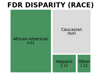
The treemap below displays precision disparity values calculated using a predefined group, in this case the ‘Caucasian’ group within the race attribute, sized based on the group size and colored based on disparity magnitude. We can see from asterisks that the disparities between the ‘Caucasian’ reference population group and both the ‘African-American’ and ‘Other’ race population groups are statistically significant at the 5% level.

Note: Groups are visualized at no less than 0.1 times the size of the reference group, and no more than 10 times the size of the reference group.

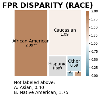
aqp.plot_disparity(bdf, group_metric='fpr_disparity', attribute_name='race', significance_alpha=0.05)

When another group, ‘Hispanic’, is the reference group, the colors change to indicate higher or lower disparity in relation to that group. Treemap square sizes may also be adjusted, as group size limits for visualization are in relation to the reference group (minimum 0.1 times reference group size and maximum 10 times the reference group size).

aqp.plot_disparity(hbdf, group_metric='fpr_disparity', attribute_name='race', significance_alpha=0.05)

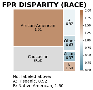
Visualizing disparities between all groups for a single user-specified disparity metric

The treemaps belows display False Positive Rate disparities calculated based on predefined reference groups (‘race’ attribute: Hispanic, ‘sex’ attribute: Male, ‘age_cat’ attribute: 25-45), sized based on group size, and colored based on disparity magnitude.

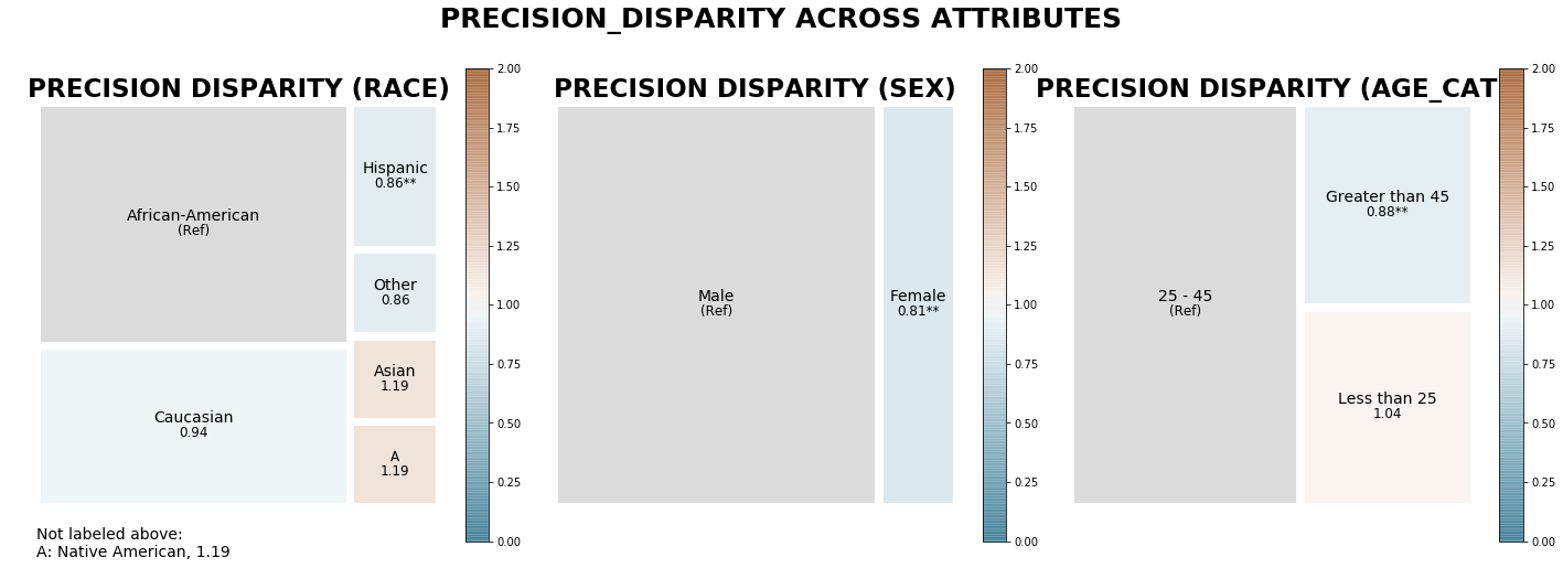
It is clear that the majority of samples in the data are African-American, male, and 25-45 for the ‘race’, ‘sex’, and age category attributes, respectively. Based on the lighter colors in the treemaps, we see that there is precision disparity relatively close to 1 (a disparity of 1 indicates no disparity) across all attributes.

j = aqp.plot_disparity_all(majority_bdf, metrics=['precision_disparity'], significance_alpha=0.05)

Visualizing disparities between groups in a single user-specified attribute for default metrics

When visualizing more than one disparity, you can specify a list of disparity metrics, 'all' disaprity metrics, or use the Aequitas default disparity metrics by not supplying an argument: - Predicted Positive Group Rate Disparity (pprev_disparity), - Predicted Positive Rate Disparity (ppr_disparity), - False Discovery Rate Disparity (fdr_disparity), - False Omission Rate Disparity (for_disparity) - False Positive Rate Disparity (fpr_disparity) - False Negative Rate Disparity (fnr_disparity)

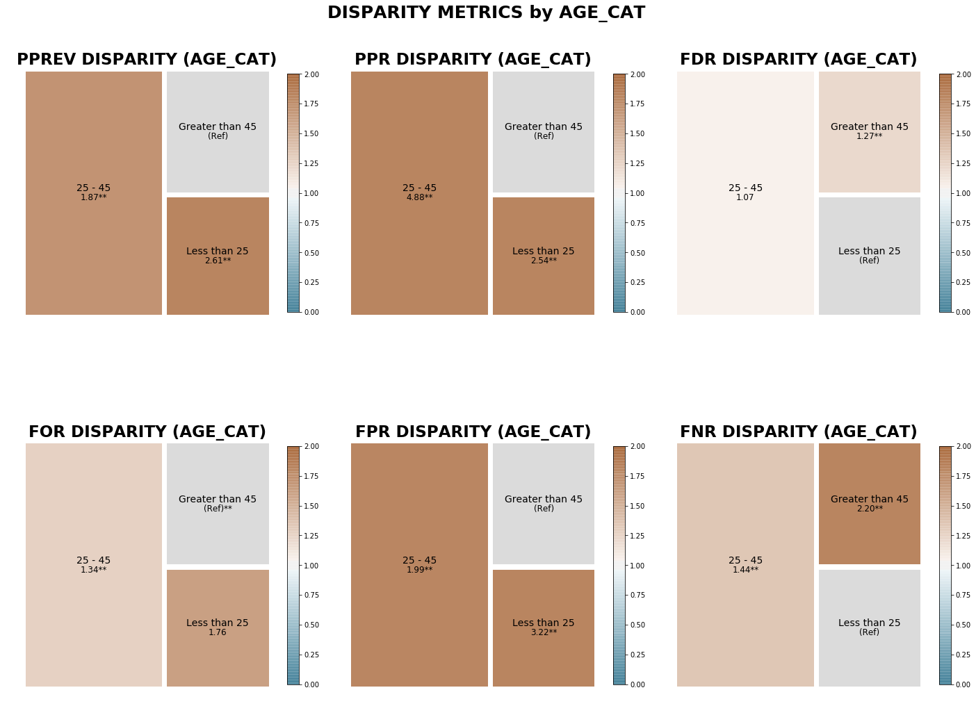
The treemaps below display the default disparities between ‘age_cat’ groups calculated based on the minimum value of each metric, colored based on disparity magnitude. We can see based on coloring that there is a lower level of false discovery rate disparity (‘fdr_disparity’) between age categories than predicted positive group rate disparity or (‘pprev_disparity’) predicted positive rate disparity (‘ppr_disparity’).

min_met = aqp.plot_disparity_all(min_metric_bdf, attributes=['age_cat'], significance_alpha=0.05)

Visualizing disparities between groups in a single user-specified attribute for all calculated disparity metrics

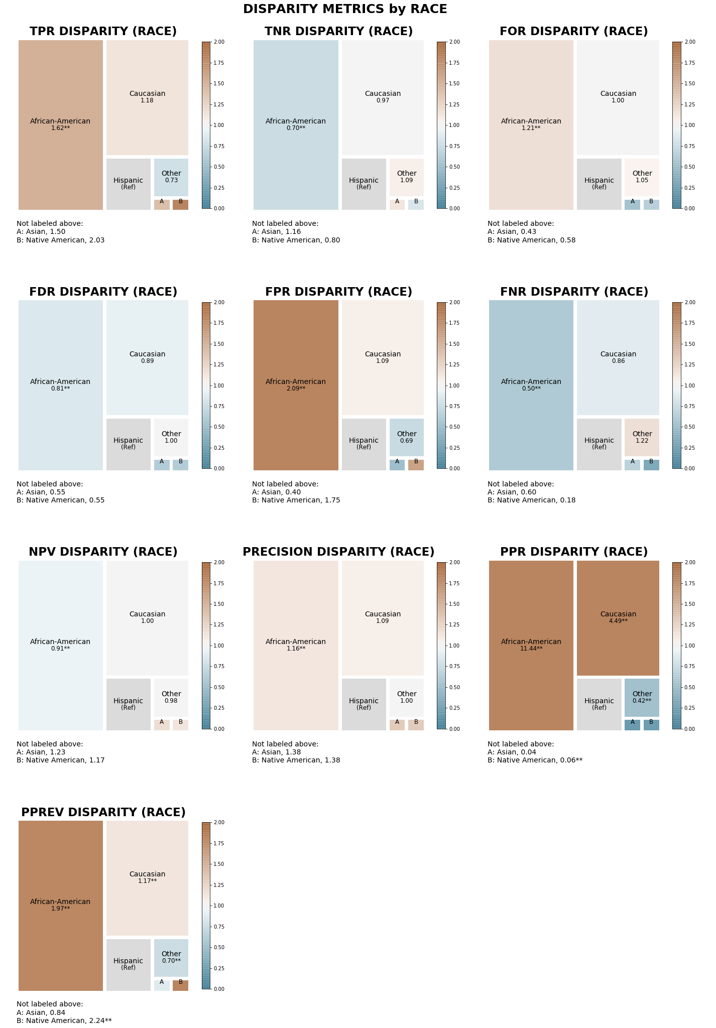
The treemaps below display disparities between ‘race’ attribute groups calculated based on predefined reference groups (‘race’ attribute: Hispanic, ‘sex’ attribute: Male, ‘age_cat’ attribute: 25-45) for all 10 disparity metrics, colored based on disparity magnitude.

tm_capped = aqp.plot_disparity_all(hbdf, attributes=['race'], metrics = 'all', significance_alpha=0.05)

Visualizing disparity between all groups for multiple user-specified disparity metrics

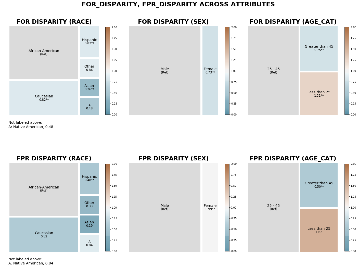
The treemaps below display False Omission Rate and False Positive Rate disparities (calculated in relation to the sample majority group for each attribute) between groups acorss all three attributes, colored based on disparity magnitude.

We see that several groups (Asian, Native American) have a much lower false omission rate than African Americans, with fairly close false omission rates between the sexes and the two older oldest age groups. Though there are many more men in the sample, the two groups have nearly identical false positive rates, while color tells us that there are larger false positive rate disparities between races and age categories than false omission rate disparity.

dp = aqp.plot_disparity_all(majority_bdf, metrics=['for_disparity', 'fpr_disparity'], significance_alpha=0.05)

Back to Top

How do I assess model fairness?

Aequitas Fairness() Class

Finally, the Aequitas Fairness() class provides three functions that provide a high level summary of fairness. This class builds on the dataframe returned from one of the three Bias() class ``get_dispariy_`` methods.

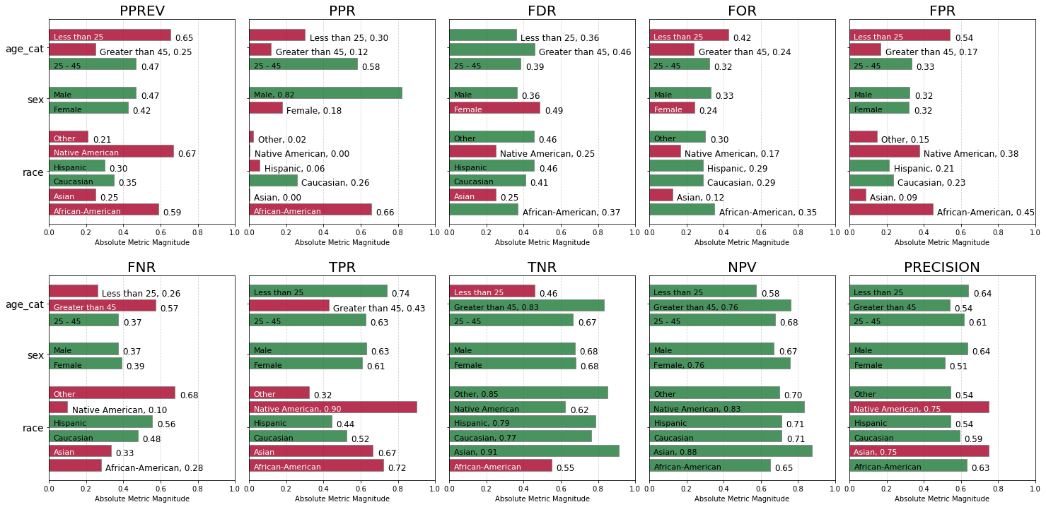
Using FPR disparity as an example and the default fairness threshold, we have:

We can assess fairness at various levels of detail:

Group Level Fairness

When the label_value column is not included in the original data set, Aequitas calculates only Statistical Parity and Impact Parities.

When the label_value is included in the original data set, the ``get_group_value_fairness()`` function builds on the previous dataframe. The ``get_group_value_fairness()`` function gives us attribute group-level statistics for fairness determinations:

Pairities Calcuated:

Parity	Column Name
True Positive Rate Parity	‘TPR Parity’
True Negative Rate Parity	‘TNR Parity’
False Omission Rate Parity	‘FOR Parity’
False Discovery Rate Parity	‘FDR Parity’
False Positive Rate Parity	‘FPR Parity’
False Negative Rate Parity	‘FNR Parity’
Negative Predictive Value Parity	‘NPV Parity’
Precision Parity	‘Precision Parity’
Predicted Positive Ratio Parity	‘Statistical Parity’
Predicted Positive Ratio Parity	‘Impact Parity’

Also assessed:

• *Type I Parity*: Fairness in both FDR Parity and FPR Parity

• *Type II Parity*: Fairness in both FOR Parity and FNR Parity

• *Equalized Odds*: Fairness in both FPR Parity and TPR Parity

• *Unsupervised Fairness*: Fairness in both Statistical Parity and Impact Parity

• *Supervised Fairness*: Fairness in both Type I and Type II Parity

• *Overall Fairness*: Fairness across all parities for all attributes

f = Fairness()
fdf = f.get_group_value_fairness(bdf)

The Fairness() class includes a method to quickly return a list of fairness determinations from the dataframe returned by the ``get_group_value_fairness()`` method.

parity_detrminations = f.list_parities(fdf)

fdf[['attribute_name', 'attribute_value'] + absolute_metrics + calculated_disparities + parity_detrminations].style

	attribute_name	attribute_value	tpr	tnr	for	fdr	fpr	fnr	npv	precision	ppr	pprev	prev	fdr_disparity	fnr_disparity	for_disparity	fpr_disparity	npv_disparity	ppr_disparity	pprev_disparity	precision_disparity	tnr_disparity	tpr_disparity	NPV Parity	TypeI Parity	Supervised Fairness	Unsupervised Fairness	Equalized Odds	Impact Parity	Statistical Parity	FOR Parity	TypeII Parity	FDR Parity	Precision Parity	FPR Parity	TPR Parity	TNR Parity	FNR Parity
0	race	African-American	0.720147	0.551532	0.34954	0.370285	0.448468	0.279853	0.65046	0.629715	0.655412	0.588203	0.51434	0.906085	0.586416	1.21315	1.91209	0.913728	2.54567	1.69022	1.0649	0.720526	1.37755	True	False	False	False	False	False	False	True	False	True	True	False	False	False	False
1	race	Asian	0.666667	0.913043	0.125	0.25	0.0869565	0.333333	0.875	0.75	0.00241182	0.25	0.28125	0.611748	0.698482	0.433839	0.370749	1.22915	0.00936768	0.718384	1.26832	1.19281	1.27525	True	False	False	False	False	False	False	False	False	False	False	False	False	True	False
2	race	Caucasian	0.522774	0.765457	0.288125	0.408665	0.234543	0.477226	0.711875	0.591335	0.257462	0.348003	0.393643	1	1	1	1	1	1	1	1	1	1	True	True	True	True	True	True	True	True	True	True	True	True	True	True	True
3	race	Hispanic	0.443966	0.785185	0.288591	0.457895	0.214815	0.556034	0.711409	0.542105	0.0572807	0.298273	0.364207	1.12046	1.16514	1.00162	0.915887	0.999346	0.222482	0.857099	0.916748	1.02577	0.849249	True	True	True	False	True	True	False	True	True	True	True	True	True	True	True
4	race	Native American	0.9	0.625	0.166667	0.25	0.375	0.1	0.833333	0.75	0.00361773	0.666667	0.555556	0.611748	0.209544	0.578453	1.59885	1.17062	0.0140515	1.91569	1.26832	0.816506	1.72158	True	False	False	False	False	False	False	False	False	False	False	False	False	True	False
5	race	Other	0.323308	0.852459	0.302013	0.455696	0.147541	0.676692	0.697987	0.544304	0.0238167	0.209549	0.352785	1.11508	1.41797	1.0482	0.629057	0.98049	0.0925059	0.602147	0.920466	1.11366	0.618447	True	False	False	False	False	False	False	True	False	True	True	False	False	True	False
6	sex	Female	0.608434	0.67893	0.242537	0.48731	0.32107	0.391566	0.757463	0.51269	0.178173	0.423656	0.356989	1.33642	1.05581	0.734738	0.990343	1.13071	0.216801	0.904348	0.806925	1.00463	0.967101	True	False	False	False	True	True	False	False	False	False	True	True	True	True	True
7	sex	Male	0.629132	0.675799	0.3301	0.364637	0.324201	0.370868	0.6699	0.635363	0.821827	0.468465	0.473105	1	1	1	1	1	1	1	1	1	1	True	True	True	True	True	True	True	True	True	True	True	True	True	True	True
8	age_cat	25 - 45	0.626257	0.666216	0.323112	0.385135	0.333784	0.373743	0.676888	0.614865	0.580042	0.46824	0.459723	1	1	1	1	1	1	1	1	1	1	True	True	True	True	True	True	True	True	True	True	True	True	True	True	True
9	age_cat	Greater than 45	0.427711	0.832096	0.241117	0.459391	0.167904	0.572289	0.758883	0.540609	0.118782	0.25	0.31599	1.1928	1.53124	0.746232	0.503031	1.12114	0.204782	0.533914	0.879232	1.24899	0.682963	True	False	False	False	False	False	False	False	False	True	True	False	False	True	False
10	age_cat	Less than 25	0.739583	0.458647	0.424528	0.36036	0.541353	0.260417	0.575472	0.63964	0.301176	0.653368	0.565075	0.935673	0.696781	1.31387	1.62187	0.850173	0.519231	1.39537	1.04029	0.688435	1.18096	True	False	False	False	False	False	False	False	False	True	True	False	True	False	False

Back to Top

How do I interpret parities?

Calling the Aequitas Fairness() class ``get_group_value_fairness()`` method on the dataframe returned from a Bias() class get_dispariy method will return the dataframe with additional columns indicating parities, as seen in the slice of the get_group_value_fairness data frame directly above.

In this case, our base groups are Caucasian for race, Male for gender, and 25-45 for age_cat. By construction, the base group has supervised fairness. (The disparity ratio is 1). Relative to the base groups, the COMPAS predictions only provide supervised fairness to one group, Hispanic.

Above, the African-American false omission and false discovery are within the bounds of fairness. This result is expected because COMPAS is calibrated. (Given calibration, it is surprising that Asian and Native American rates are so low. This may be a matter of having few observations for these groups.)

On the other hand, African-Americans are roughly twice as likely to have false positives and 40 percent less likely to false negatives. In real terms, 44.8% of African-Americans who did not recidivate were marked high or medium risk (with potential for associated penalties), compared with 23.4% of Caucasian non-reoffenders. This is unfair and is marked False below.

These findings mark an inherent trade-off between FPR Fairness, FNR Fairness and calibration, which is present in any decision system where base rates are not equal. See Chouldechova (2017). Aequitas helps bring this trade-off to the forefront with clear metrics and asks system designers to make a reasoned decision based on their use case.

Attribute Level Fairness

Use the ``get_group_attribute_fairness()`` function to view only the calculated parities from the ``get_group_value_fairness()`` function at the attribute level.

gaf = f.get_group_attribute_fairness(fdf)
gaf

	model_id	score_threshold	attribute_name	Statistical Parity	Impact Parity	FDR Parity	FPR Parity	FOR Parity	FNR Parity	TPR Parity	TNR Parity	NPV Parity	Precision Parity	TypeI Parity	TypeII Parity	Equalized Odds	Unsupervised Fairness	Supervised Fairness
0	1	binary 0/1	age_cat	False	False	True	False	False	False	False	False	True	True	False	False	False	False	False
1	1	binary 0/1	race	False	False	False	False	False	False	False	False	True	False	False	False	False	False	False
2	1	binary 0/1	sex	False	True	False	True	False	True	True	True	True	True	False	False	True	False	False

Overall Fairness

The ``get_overall_fairness()`` function gives a quick boolean assessment of the output of ``get_group_value_fairness()`` or ``get_group_attribute_fairness()``, returning a dictionary with a determination across all attributes for each of: - Unsupervised Fairness - Supervised Fairness - Overall Fairness

gof = f.get_overall_fairness(fdf)
gof

{'Unsupervised Fairness': False,
 'Supervised Fairness': False,
 'Overall Fairness': False}

Back to Top

How do I visualize bias metric parity?

Once you have run the Group() class to retrieve a crosstab of absolute group value bias metrics, added calculdated disparities via one of the the Bias() class ``get_disparity`` functions, and added parity determinations via the Fairness() class ``get_group_value_fairness()`` or ``get_group_attribute_fairness()`` method, you are ready to visualize biases and disparities in terms of fairness determination.

For visualizing absolute metric fairness with the the Aequitas Plot() class, a particular metric can be specified with ``plot_fairness_group()``. A list of particular metrics of interest or ‘all’ metrics can be plotted with ``plot_fairness_group_all()``.

Visualizing parity of a single absolute group metric across all population groups

The chart below displays absolute group metric Predicted Positive Rate Disparity (ppr) across each attribute, colored based on fairness determination for that attribute group (green = ‘True’ and red = ‘False’).

We can see from the green color that only the 25-45 age group, Male category, and Caucasian groups have been determined to be fair. Sound familiar? They should! These are the groups selected as reference groups, so this model is not fair in terms of Statistical Parity for any of the other groups.

z = aqp.plot_fairness_group(fdf, group_metric='ppr')

Visualizing all absolute group metrics across all population groups

The charts below display all calculated absolute group metrics across each attribute, colored based on fairness determination for that attribute group (green = ‘True’ and red = ‘False’).

Immediately we can see that negative predictive parity status is ‘True’ for all population groups, and that only two groups had a ‘False’ determination for true negative parity.

fg = aqp.plot_fairness_group_all(fdf, ncols=5, metrics = "all")

Back to Top

How do I visualize parity between groups in my model?

To visualize disparity fairness based on the dataframe returned from the Fairness() class ``get_group_value_fairness()`` method, a particular disparity metric can be specified with the ``plot_fairness_disparity()`` method in the the Aequitas Plot() class. To plot a single disparity, a metric and an attribute must be specified.

Disparities related to a list of particular metrics of interest or 'all' metrics can be plotted with ``plot_fairness_disparity_all()``. At least one metric or at least one attribute must be specified when plotting multiple fairness disparities (or the same disparity across multiple attributes).

Visualizing parity between groups in a single user-specified attribute for all calculated disparity metrics

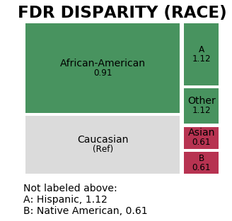
The treemap below displays False Discovery Rate disparity values between race attribute groups calculated based on a predefined reference group (‘Caucasian’), colored based on fairness determination for that attribute group (green = ‘True’ and red = ‘False’). We see very quickly that only two groups have a ‘False’ parity determination.

m = aqp.plot_fairness_disparity(fdf, group_metric='fdr', attribute_name='race')

Researcher Check: Could the unfairness I am seeing be related to small group sizes in my sample?

Use the min_group parameter on all visualization methods to vizualize parities for only those sample population groups above a user-specified percentage of the total sample size. Note that only the smallest groups had an ‘False’ determination for false discovery rate parity above. The parity determination is ‘True’ for all groups at least 1% of the sample size .

m = aqp.plot_fairness_disparity(fdf, group_metric='fdr', attribute_name='race',
                                min_group_size=0.01, significance_alpha=0.05)

Visualizing parity between groups in a single user-specified attribute for all calculated disparity metrics

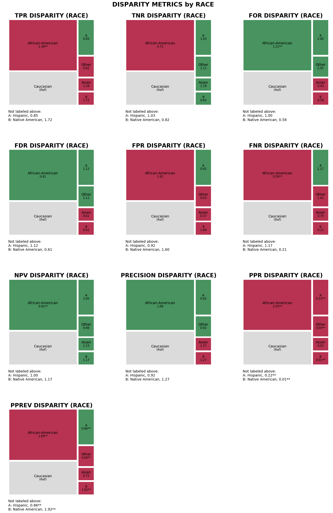
The treemaps below display disparities between race attribute groups calculated based on a predefined reference group (‘Caucasian’) for all 10 disparity metrics, colored based on fairness determination for that attribute group (green = ‘True’ and red = ‘False’).

As all treemap squares are sized and positioned based on group size, the population groups on all subplots are found in the same place across all disparity metrics, allowing for ease of comparison of fairness determinations for each ‘race’ group across every calculated dipsarity metric.

a_tm = aqp.plot_fairness_disparity_all(fdf, attributes=['race'], metrics='all',
                                       significance_alpha=0.05)

Visualizing parity between all groups for multiple user-specified disparity metrics

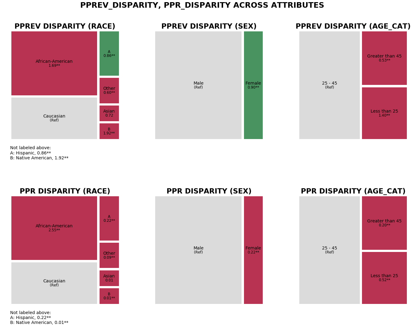
The treemaps below display Predicted Positive Group Rate (pprev) and Predicted Positive Rate (ppr) disparities between attribute groups for all three attributes (race, sex, age category) calculated based on predefined reference groups (‘race’ attribute: Caucasian, ‘sex’ attribute: Male, ‘age_cat’ attribute: 25-45), colored based on fairness determination for that attribute group (green = ‘True’ and red = ‘False’). As we want to plot for all groups, there is no need to specify any attributes.

We can see that the Predicted Positive Group Rate Parity (Impact Parity) determination was ‘False’ for nearly every race in comparison to Caucausians, and ‘False’ for every other age category in comparison to the 25-45 age group, and that overall Predicted Positive Rate Parity (Statistical Parity) did not have any ‘True’ fairness determinations at all.

r_tm = aqp.plot_fairness_disparity_all(fdf, metrics=['pprev_disparity', 'ppr_disparity'],
                                       significance_alpha=0.05)

Visualizing parity between groups in multiple user-specified attributes

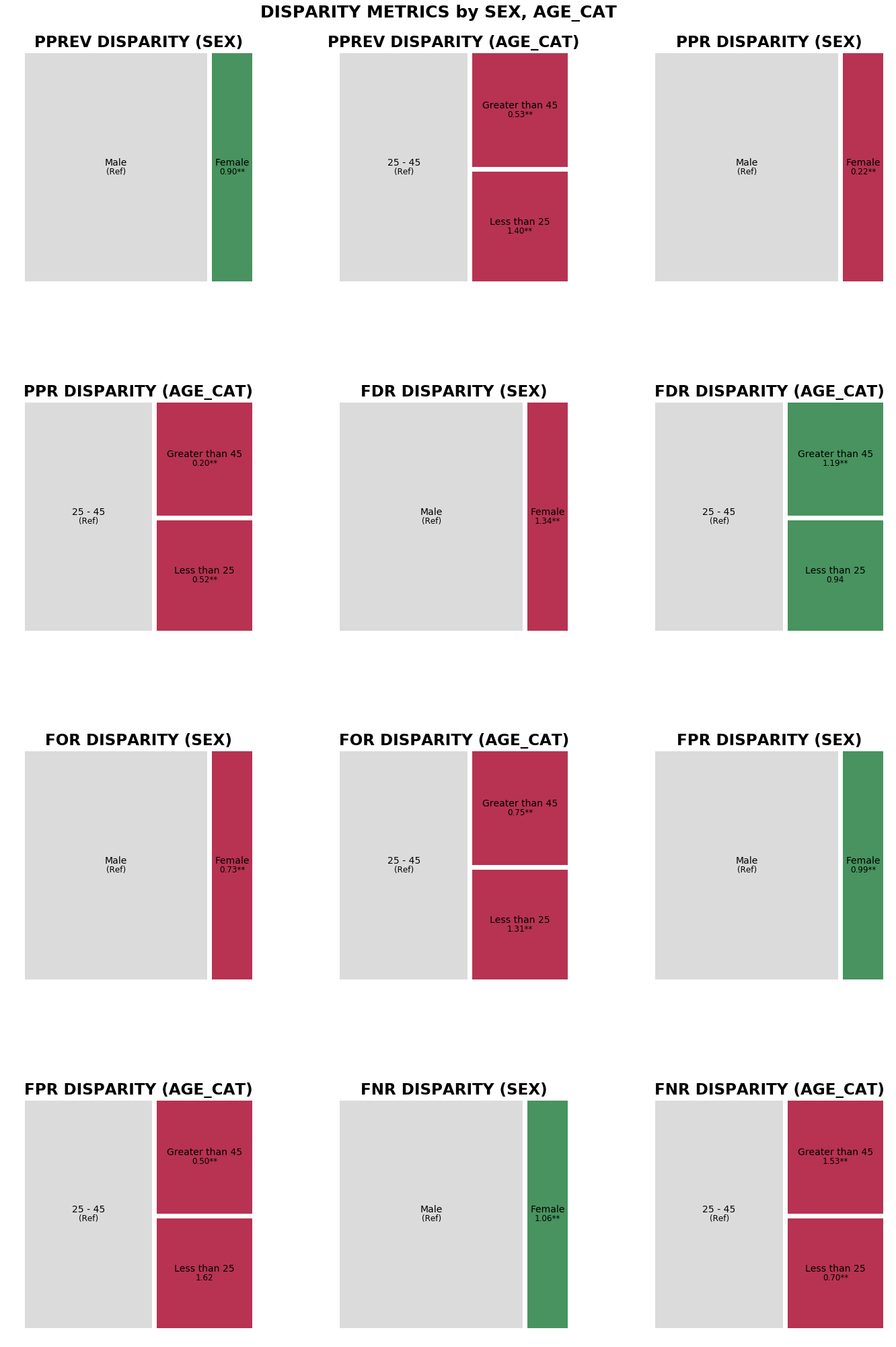
The treemaps below display disparities between attribute groups for all two attributes (sex, age category) calculated based on predefined reference groups (‘sex’ attribute: Male, ‘age_cat’ attribute: 25-45) for the six default disparity metrics, colored based on fairness determination for that attribute group (green = ‘True’ and red = ‘False’). As we want to see only the default metrics, we do not need to set the ‘metrics’ parameter.

Note that there is slightly more parity between the sexes (FNR, FDR, FNR, and Statistical Parity) than between age categories (FDR Parity only).

n_tm = aqp.plot_fairness_disparity_all(fdf, attributes=['sex', 'age_cat'],
                                       significance_alpha=0.05)

The Aequitas Effect

By breaking down the COMPAS predictions using a variety of bias and disparity metrics calculated using different reference groups, we are able to surface the specific metrics for which the model is imposing bias on given attribute groups, and have a clearer lens when evaluating models and making recommendations for intervention.

Researchers utilizing Aequitas will be able to make similar evaluations on their own data sets, and as they continue to use the tool, will begin to identify patterns in where biases exist and which models appear to produce less bias, thereby helping to reduce bias and its effects in future algorithm-based decision-making.

Back to Top