

Spatial analytics: PostGIS Workshop

Slides

• Tutorial slides (2016)

A little bit of theory

Spatial database

• Storage of spatial data
• Analysis of geographic data
• Manipulation of spatial objects just like the other database objects
  • Creation of subsets of data
  • Fixing geographic data
  • $\ldots$
• Database backend for apps

Spatial data

• Data which describes or represents either a location or a shape

• Points, lines, polygons

• Besides the geometrical properties, the spatial data has attributes.

• Examples:

  • Geocodable address
  • Crime patterns
  • EMS / patient location
  • Weather information
  • City planning
  • Hazard detection

Relationships

• Proximity
• Adjacency (touching, connectivity)
• Containment

Operations

• Area
• Length
• Intersection
• Union
• Buffer

Why a db instead of a file?

Spatial data is usually related to other types of data.

How load data to the db?

• shp2pgsql

  • imports standard esri shapefiles and dbf

• ogr2ogr

  • imports 20 different vector and flat files

The spatial data that is not spatial data

longitude	latitude	disease	date
26.870436	-31.909519	mumps	13/12/2008
26.868682	-31.909259	mumps	24/12/2008
26.867707	-31.910494	mumps	22/01/2009
26.854908	-31.920759	measles	11/01/2009
26.855817	-31.921929	measles	26/01/2009
26.852764	-31.921929	measles	10/02/2009
26.854778	-31.925112	measles	22/02/2009
26.869072	-31.911988	mumps	02/02/2009

(the disease and date columns are the attributes of this data)

shape files

• Stored in files on the computer
• The most common one is probably the 'shape file'
  • It consists of at least three different files that work together to store vector data

extension	description
`.shp`	the geometry file
`.dbf`	the attributes file
`.shx`	index file

Vector data

• Is stored as a series of x,y coordinate pairs inside the computer's memory.
• Vector data is used to represent points (1 vertex) , lines (polyline) (2 or more vertices, but the first and the last one are different) and areas (polygons).
• A vector feature has its shape represented using geometry.
• The geometry is made up of one or more interconnected vertices.
• A vertex describes a position in space using an x, y and optionally z axis.
• The x and y values will depend on the coordinate reference system (CRS) being used.

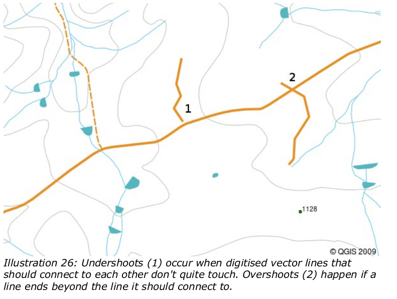
Problems with vector data

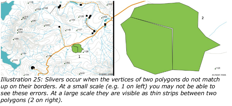Image from A gentle introduction to gis Sutton T., Dassau O., Sutton M. 2009

"Image from A gentle introduction to gis Sutton T., Dassau O., Sutton M. 2009

Raster data

• Stored as a grid of values
• Each cell or pixel represents a geographical region, and the value of the pixel represents some attribute of the region
• Use it when you want to represent a continuous information across an area
• Multi-band images, each band contains different information

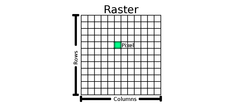Image from A gentle introduction to gis Sutton T., Dassau O., Sutton M. 2009

Problems with raster data

High resolution raster data requires a huge amount of computer storage.

Exercise: Cleaning and exploring spatial data

Connect to the db

host:  gis-tutorial.c5faqozfo86k.us-west-2.rds.amazonaws.com
port: 5432
username: dssg_gis
password: dssg-gis
db name:gis_tutorial

SSH Tunneling

ssh -fNT -L \
    8889:gis-tutorial.c5faqozfo86k.us-west-2.rds.amazonaws.com:5432  \
    -i ~/.ssh/your-dssh-key ec2-instance.dssg.io  ## ssh tunneling

Command line client

psql -h localhost -p 8889 -U dssg_gis  gis_tutorial

Setup

• create an schema using your github account
  • (mine is nanounanue)

    create schema your-github-username;

Upload the first shapefiles

• There are several shapefiles in the data directory

• First, we can see some information from the files

  ogrinfo -al roads.shp

Observe that the projection is

...
projcs["nad83_massachusetts_mainland",
    geogcs["gcs_north_american_1983",
        datum["north_american_datum_1983",
            spheroid["grs_1980",6378137,298.257222101]],
        primem["greenwich",0],
        unit["degree",0.017453292519943295]],
    projection["lambert_conformal_conic_2sp"],
    parameter["standard_parallel_1",42.68333333333333],
    parameter["standard_parallel_2",41.71666666666667],
    parameter["latitude_of_origin",41],
    parameter["central_meridian",-71.5],
    parameter["false_easting",200000],
    parameter["false_northing",750000],
    unit["meter",1]]
...

This projection measures the area in meters. but

• Using shp2psql tool upload the following files: roads, land, hydrology

  shp2psql --host=localhost --port=8889 --username=dssg_gis \
   -f roads.shp gis your-github-username.roads \
   | psql -h localhost -p 8889 -u dssg_gis  gis_tutorial
  ## if you want to change the projection to wgs 1984 (the one used in google maps)
  ## you need to add the flag -s 26986:4326 before the name of the database (gis)
  

If you open QGIS you should see something like the following:

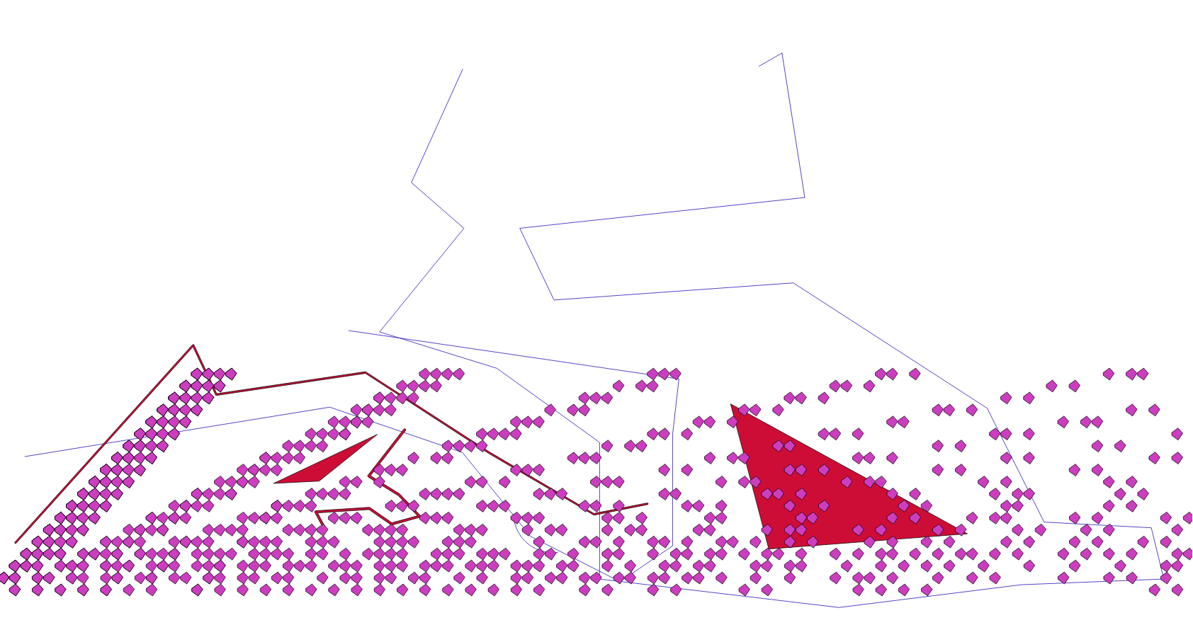Figure: land (purple), hydrology (red) and roads (blue) after their insertion in the database

and after some customization:

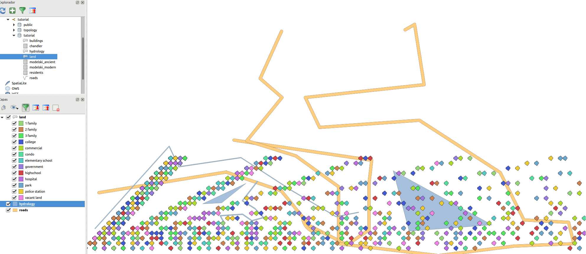Figure: After adjusting the style in QGIS: land (one color per type), hydrology (blue) and roads (yellow)

note that we have lands over the roads and over the water.

Spatial predicates for cleaning

• We will use st_intersects() and st_dwithin() for removing the land which is touch with roads and water, and if it is too far of roads and water, respectively

• See the file for the sql statements.

• NOTE: For use of the EXISTS(subquery) look here and here

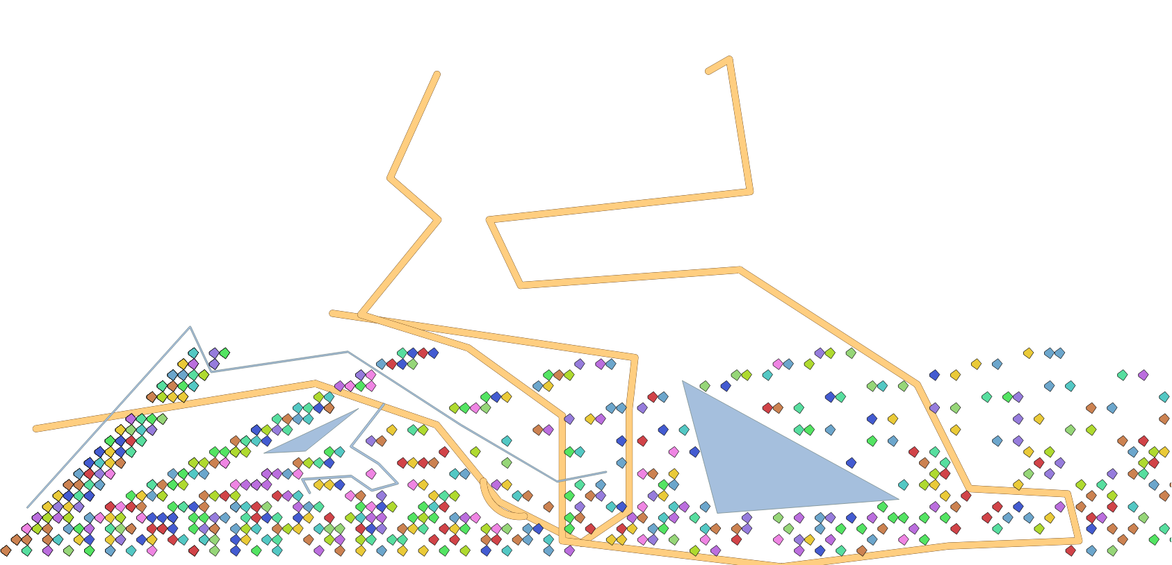Figure: After removing the land objects which intersects roads or water or where too far from those

• St_intersects(a,b) returns true if exists at least one point in common between the geometrical objects a and b.

• St_dwithin(a,b,distance) returns true if the geometries a and b are within the specified distance of one another.

• Other functions: st_equals, st_disjoint, st_touches, st_crosses, st_overlaps, st_contains.

Add more data: buildings and residents

Upload to the database the shapefiles buildings and residents.

## This time I will use ogr2ogr, but this is for demostration purpose only
## It is easier use shp2pgsql
ogr2ogr -f "PostgreSQL" \
 PG:"host=localhost user=dssg_gis dbname=gis_tutorial password=dssg-gis port=8889" \
  buildings.shp -nln your-github-username.buildings

Spatial joins: creating new views

• As you can see, is not a spatial data. It is a regular psv file. But it contains the pid of the land in which the resident lives.

  csvhead -d '|' ./data/my_town/residents.psv | head

How can I convert this data in spatial data?

    select
    r.*  -- All the attributes of resident
    , st_centroid(l.the_geom) -- The centroid of the land in which this resident lives
    from
    residents as r
    inner join -- only the matches
    land as l
    on
    r.pid = l.pid;

Ok, very well. But, How can I see this new "data" in QGIS? You need to create a view

    create or replace view residents_loc
    as
    select
    row_number() over() as rl_id -- We need an unique identifier
    , r.*  -- All the attributes of resident
    , st_centroid(l.the_geom) as the_geom -- The centroid of the land in which this resident lives
    from
    residents as r
    inner join -- only the matches
    land as l
    on
    r.pid = l.pid;

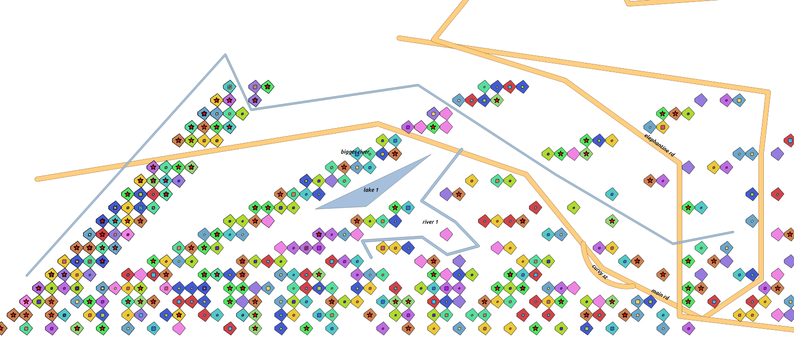Figure: After the creation of the view residents_loc (red star)

Spatial operations: Legal issues in our town

How much real state area do we have?

    select
    sum(st_area(the_geom))/1000000 as total_sq_km
    , st_area(st_union(the_geom))/1000000 as no_overlap_total_sq_km
    -- st_union dissolves the overlaps!
    from land;

Oh, oh. And buildings?

    select
    sum(st_area(the_geom))/1000000 as total_sq_km
    , st_area(st_union(the_geom))/1000000 as no_overlap_total_sq_km
    from buildings;

- We have buildings inside buildings, and some lands overlaps with other lands :(

• Other operations: st_intersection(a,b), st_difference(a,b), st_symdifference(a,b), st_buffer(c), st_convexhull(c)

Spatial joins: Which lands intersects?

    select
    p.pid -- the land
    , count(o.pid) as total_intersections -- qty of intersections
    , array_agg(o.pid) as intersected_parcels -- the other lands
    from
    land as p
    inner join
    land as o
    on
    (p.pid <> o.pid and st_intersects(p.the_geom, o.the_geom))
    group by p.pid
    order by p.pid;
    -- First row returned: pid IN ('000000225', '000027745','000092727','000057051')

Which type of overlap?

    select
    count(o.pid) as total_intersections
    -- Overlaps?
    , count(case when st_overlaps(o.the_geom,p.the_geom) then 1 else null end) as o_overlaps_p
    -- It is the same?
    , count(case when st_equals(o.the_geom,p.the_geom) then 1 else null end) as o_equals_p
    from land as p
    inner join land as o
    on (p.pid <> o.pid and st_intersects(p.the_geom, o.the_geom));

• st_overlaps(a,b) returns true if the geometries share some but not all the points, and the intersection has the same dimension as a, b

Cleaning the mess: Reassigning residents

    update residents
    set pid = a.newpid
    from (
    select p.pid, min(o.pid) as newpid
    from land as p
    inner join
    land as o on
    (p.pid = o.pid or st_equals(p.the_geom, o.the_geom))
    group by p.pid
    having p.pid <> min(o.pid)) as a
    where residents.pid = a.pid
    returning * -- Return all the updated residents
    -- so you can see what you just do
    -- (or you can store it in a another table using CTAS)

Cleaning the mess: Deleting the dupe land

    -- Add a new column for storing the house types
    alter table land add column land_type_other varchar[];

    -- Copy the types to the first parcel
    update land
    set land_type_other = a.dupe_types
    from (
    select p.pid
    , min(o.pid) as newpid
    , array_agg(distinct o.land_type) as dupe_types
    from land as p
    inner join land as o
    on
    (st_equals(p.the_geom, o.the_geom))
    group by p.pid
    having count(p.pid) > 1 and p.pid = min(o.pid)
    ) as a
    where land.pid = a.pid
    returning *;

    -- Delete the parcels
    delete from land
    where pid in
    (select p.pid
    from land as p inner join land as o on
    (st_equals(p.the_geom, o.the_geom))
    group by p.pid
    having count(p.pid) > 1 and p.pid <> min(o.pid)) ;

Spatial analytics: Questions

How many kinds under 12 are further than a km of an elementary school?

    select
    sum(num_children_b12)*100.00/(select sum(num_children_b12) from residents)
    from residents as r
    inner join land as l on r.pid = l.pid
    left join (
    select pid, the_geom from land
    where
    land_type = 'elementary school'
    or
    'elementary school' = any(land_type_other)
    ) as eschools
    on st_dwithin(l.the_geom, eschools.the_geom, 1000)
    where eschools.pid is null;

How much area are in empty lands?

    select st_area(st_union(the_geom))/1000000
    from land
    where
    land_type = 'vacant land';

Which are the 10 nearest houses to the lakes?

    select h.hyd_name,
    array(
    select bldg_name
    from buildings b
    where
    b.bldg_type like '%family'
    order by h.the_geom <#> b.the_geom limit 5
    )
    from hydrology h
    where h.hyd_name in  ('lake 1', 'elephantine youth');

• Note the <#> (bounding box), <-> (centroids) are distance operators, see here and here.

Exercise: Mapping civilizations

Intro

• Recently this article was published: Spatializing 6,000 years of global urbanization from 3700 BC to AD 2000 Reba, M., Reitsma, F. and Seto, C., 2016
• The article describes all the cities since 3700 BC, including name, population and the position (latitude, longitude).
• We will use a subset (chandlerV2) of the data for transforming it to a table, and then generating a geojson.

Uploading the data

• Run the following inside ./data/Historical Urban Population Growth Data

  cvslook chandlerV2.csv

• It will fail due some encoding issues

  iconv -f iso-8859-1 -t utf-8 chandlerV2.csv > chandler_utf8.csv
  csvsql --db postgresql://dssg_gis:dssg-gis@localhost:8889/gis_tutorial \
  --insert chandlerV2_utf8.csv --table chandler --db-schema nanounanue
  

SQL stuff

    select count(*) from chandler;  -- How many cities do we have?

Let’s create a new table for easier manipulation

    create table cities as -- CTAS
    select
    "City" as city,
    "Country" as country,
    "Latitude" as y_lat,
    "Longitude" as x_lon from chandler;

Adding a geometry column and transform to Point

    alter table cities add column geom geometry(Point, 4326);
    -- Transforming Lon/Lat to Points
    update cities set geom = ST_SetSRID(ST_MakePoint(x_lon, y_lat), 4326);

Converting to GeoJSON

    \copy (
     select row_to_json(fc)
     from (
        select 'featurecollection' as type, array_to_json(array_agg(f)) as features
        from (
          select 'feature' as type
          , st_asgeojson(cities.geom)::json as geometry
          , row_to_json(
            (select c from (select city, country) as c)
          ) as properties
          from cities
        ) as f
      )  as fc)
    to '~/cities.geojson';

• This type of file could be used with d3.js for making interactive plots.

• For better performance you could use topojson

More resources!

• PostGIS: More about spatial queries
• Exploratory spatial data analysis with Python and PostGIS