An Early Intervention System: Chicago food inspections#

Before continue, Did you…?

This case study, part of the dirtyduck tutorial, assumes that you already setup the tutorial’s infrastructure and load the dataset.

If you didn’t setup the infrastructure go here,
If you didn't load the data, you can do it very quickly or you can follow all the steps and explanations about the data.

Problem description#

Triage is designed to build, among other things, early warning systems (also called early intervention, EIS). While there are several differences between modeling early warnings and inspection prioritization, perhaps the biggest differences is that the entity is active (i.e. it is doing stuff for which an outcome will happen) in EIS, but passive (e.g it is inspected) in resource prioritization. Among other things, this difference affects the way the outcome is built.

Saying that, here's the question we want to answer:

Will my restaurant be inspected in the next $Y$ period of time?

Where $X$ could be 3 days, 2 months, 1 year, etc.

We will translate that problem to

Will my restaurant be at the top- $X$ facilities most likely to be inspected in the next $Y$ period of time?

Knowing the answer to this question enables you (as the restaurant owner or manager) to prepare for the inspection.

What are the outcomes?#

The trick to note is that on any given day there are two possible outcomes: the facility was inspected and the facility wasn't inspected. Our outcomes table will be larger than in the resource prioritization example because we need an outcome for every active facility on every date. The following image tries to exemplify this reasoning:

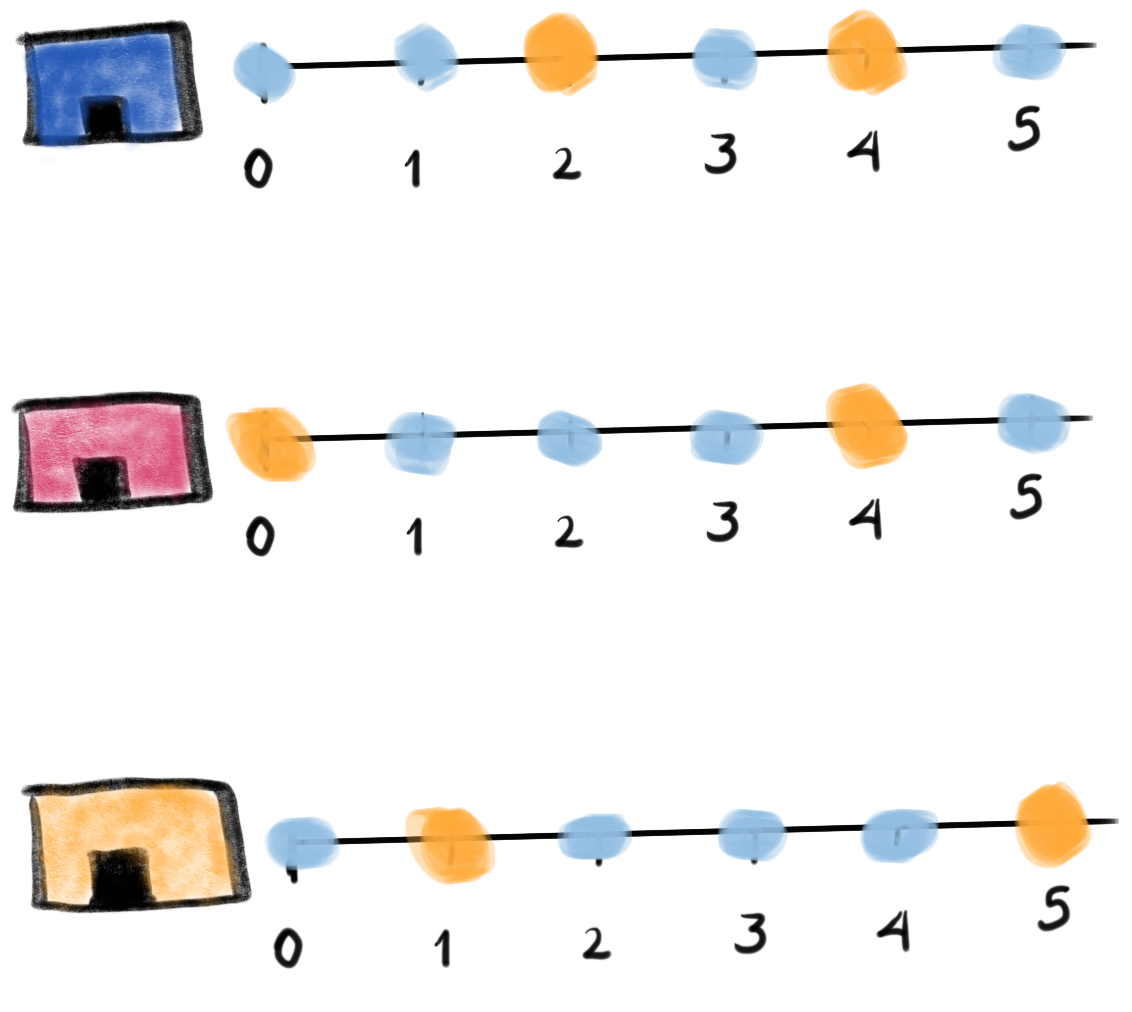Figure. The image shows three facilities (blue, red and orange), and next to each, a temporal line with 6 days (0-5). Each dot represents the event (whether an inspection happened). Yellow means the inspection happened (TRUEoutcome) and blue means it didn't (FALSE outcome). Each facility in the image had two inspections, six in total.

Fortunately, triage will help us to create this table.

What are the entities of interest? The cohort#

We are interested in predict only in active facilities (remember, in this case study, you own a restaurant, What is the point on predict if your restaurant is already closed for good?). This is the same cohort as the cohort table in the resource prioritization case study

Experiment description file

You could check the meaning about experiment description files (or configuration files) in A deeper look into triage.

First the usual stuff. Note that we are changing model_comment and label_definition (remember that this is used for generating the hash that differentiates models and model groups).

config_version: 'v8'

model_comment: 'eis: 01'
random_seed: 23895478

user_metadata:
  label_definition: 'inspected'
  experiment_type: 'eis'
  description: |
    EIS 01
  purpose: 'model creation'
  org: 'DSaPP'
  team: 'Tutorial'
  author: 'Your name here'
  etl_date: '2019-05-07'

model_group_keys:
  - 'class_path'
  - 'parameters'
  - 'feature_names'
  - 'feature_groups'
  - 'cohort_name'
  - 'state'
  - 'label_name'
  - 'label_timespan'
  - 'training_as_of_date_frequency'
  - 'max_training_history'
  - 'label_definition'
  - 'experiment_type'
  - 'org'
  - 'team'
  - 'author'
  - 'etl_date'

For the labels the query is pretty simple, if the facility showed in the data, it will get a positive outcome, if not they will get a negative outcome

label_config:
  query: |
    select
    entity_id,
    True::integer as outcome
    from semantic.events
    where '{as_of_date}'::timestamp <= date
    and date < '{as_of_date}'::timestamp + interval '{label_timespan}'
    group by entity_id
  include_missing_labels_in_train_as: False
  name: 'inspected'

Note the two introduced changes in this block, first, the outcome is True , because all our observations represent inspected facilities (see discussion above and in particular previous image), second, we added the line include_missing_labels_in_train_as: False. This line tells triage to incorporate all the missing facilities in the training matrices with False as the label.

As stated we will use the same configuration block for cohorts that we used in inspections:

cohort_config:
  query: |
    select e.entity_id
    from semantic.entities as e
    where
    daterange(start_time, end_time, '[]') @> '{as_of_date}'::date
  name: 'active_facilities'

Modeling Using Machine Learning#

We need to specify the temporal configuration, this section should reflect the operationalization of the model.

Let’s assume that every facility owner needs 6 months to prepare for an inspection. So, the model needs to answer the question: Will my restaurant be inspected in the next 6 months?

Temporal configuration#

    temporal_config:
        feature_start_time: '2010-01-04'
        feature_end_time: '2018-06-01'
        label_start_time: '2014-06-01'
        label_end_time: '2018-06-01'

        model_update_frequency: '6month'
        training_label_timespans: ['6month']
        training_as_of_date_frequencies: '6month'

        test_durations: '6month'
        test_label_timespans: ['6month']
        test_as_of_date_frequencies: '6month'

        max_training_histories: '5y'

As before, you can generate the image of the temporal blocks:

# Remember to run this in bastion  NOT in your laptop shell!
triage experiment experiments/eis_01.yaml --show-timechop

What? … Bastion?

bastion is the docker container that contains all the setup required to run this tutorial, if this is the first time that you see this word, you should stop and revisit setup infrastructure.

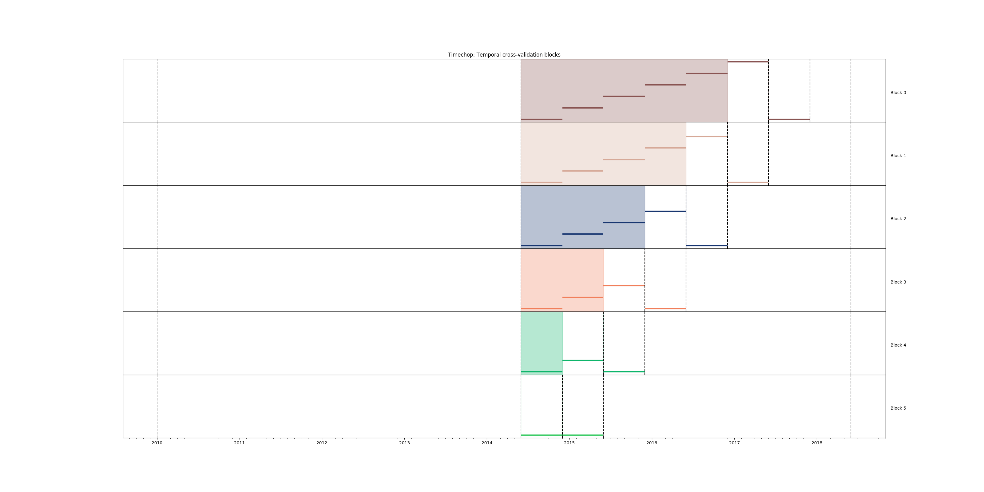Figure. Temporal blocks for the Early Warning System. We want to predict the most likely facilities to be inspected in the following 6 months

Features#

Regarding the features, we will use the same ones that were used in inspections prioritization:

    feature_aggregations:
      -
        prefix: 'inspections'
        from_obj: 'semantic.events'
        knowledge_date_column: 'date'

        aggregates_imputation:
          count:
            type: 'zero_noflag'

        aggregates:
          -
            quantity:
              total: "*"
            metrics:
              - 'count'

        intervals: ['1month', '3month', '6month', '1y', 'all']

      -
        prefix: 'risks'
        from_obj: 'semantic.events'
        knowledge_date_column: 'date'

        categoricals_imputation:
          sum:
            type: 'zero'
          avg:
            type: 'zero'

        categoricals:
          -
            column: 'risk'
            choices: ['low', 'medium', 'high']
            metrics:
              - 'sum'
              - 'avg'

        intervals: ['1month', '3month', '6month', '1y', 'all']

      -
        prefix: 'results'
        from_obj: 'semantic.events'
        knowledge_date_column: 'date'

        categoricals_imputation:
          all:
            type: 'zero'

        categoricals:
          -
            column: 'result'
            choice_query: 'select distinct result from semantic.events'
            metrics:
              - 'sum'
              - 'avg'

        intervals: ['1month', '3month', '6month', '1y', 'all']

      -
        prefix: 'inspection_types'
        from_obj: 'semantic.events'
        knowledge_date_column: 'date'

        categoricals_imputation:
          sum:
            type: 'zero_noflag'

        categoricals:
          -
            column: 'type'
            choice_query: 'select distinct type from semantic.events where type is not null'
            metrics:
              - 'sum'

        intervals: ['1month', '3month', '6month', '1y', 'all']

We specify that we want to use all possible feature-group combinations for training:

    feature_group_definition:
       prefix:
         - 'inspections'
         - 'results'
         - 'risks'
         - 'inspection_types'

    feature_group_strategies: ['all']

i.e. all will train models with all the features groups, leave-one-in will use only one of the feature groups for traning, and lastly, leave-one-out will train the model with all the features except one.

Algorithm and hyperparameters#

We will begin defining some basic models as baselines.

'triage.component.catwalk.baselines.thresholders.SimpleThresholder':
  rules:
    - ['inspections_entity_id_1month_total_count > 0']
    - ['results_entity_id_1month_result_fail_sum > 0']
    - ['risks_entity_id_1month_risk_high_sum > 0']

'triage.component.catwalk.baselines.rankers.PercentileRankOneFeature':
  feature: ['risks_entity_id_all_risk_high_sum', 'inspections_entity_id_all_total_count', 'results_entity_id_all_result_fail_sum']
  low_value_high_score: [True]

'sklearn.dummy.DummyClassifier':
  strategy: ['prior', 'stratified']

'sklearn.tree.DecisionTreeClassifier':
  criterion: ['gini']
  max_features: ['sqrt']
  max_depth: [1,2,5,~]
  min_samples_split: [2]

'triage.component.catwalk.estimators.classifiers.ScaledLogisticRegression':
  penalty: ['l1','l2']
  C: [0.000001, 0.0001, 0.01,  1.0]

How did I know the name of the features?

triage has a very useful utility called featuretest

    triage featuretest experiments/eis_01.yaml 2018-01-01

You can use for testing the definition of your features and also to see if the way that the features are calculated is actually what do you expect.

Here we are using it just to check the name of the generated features.

triage will create 20 model groups: algorithms and hyperparameters (4 DecisionTreeClassifier, 8 ScaledLogisticRegression, 2 DummyClassifier, 3 SimpleThresholder and 3 PercentileRankOneFeature) × 1 features sets (1 all). The total number of models is three times that (we have 6 time blocks, so 120 models).

    scoring:
        testing_metric_groups:
            -
              metrics: [precision@, recall@]
              thresholds:
                percentiles: [1.0, 2.0, 3.0, 4.0, 5.0, 10, 15, 20, 25, 30, 35, 40, 45, 50, 55, 60, 65, 70, 75, 80, 85, 90, 95, 100]
                top_n: [1, 5, 10, 25, 50, 100, 250, 500, 1000]


        training_metric_groups:
          -
            metrics: [accuracy]
          -
            metrics: [precision@, recall@]
            thresholds:
              percentiles: [1.0, 2.0, 3.0, 4.0, 5.0, 10, 15, 20, 25, 30, 35, 40, 45, 50, 55, 60, 65, 70, 75, 80, 85, 90, 95, 100]
              top_n: [1, 5, 10, 25, 50, 100, 250, 500, 1000]

As a last step, we validate that the configuration file is correct:

# Remember to run this in bastion  NOT in your laptop shell!
triage experiment experiments/eis_01.yaml  --validate-only

And then just run it:

# Remember to run this in bastion  NOT in your laptop shell!
time triage experiment experiments/eis_01.yaml

Protip

We are including the command time in order to get the total running time of the experiment. You can remove it, if you like.

This will take a lot amount of time (on my computer took 3h 42m), so, grab your coffee, chat with your coworkers, check your email, or read the DSSG blog. It's taking that long for several reasons:

There are a lot of models, parameters, etc.
We are running in serial mode (i.e. not in parallel).
The database is running on your laptop.

You can solve 2 and 3. For the second point you could use the docker container that has the multicore option enabled. For 3, I recommed you to use a PostgreSQL database in the cloud, such as Amazon's PostgreSQL RDS (we will explore this later in running triage in AWS Batch).

After the experiment finishes, we can create the following table:

    with features_groups as (
    select
        model_group_id,
        split_part(unnest(feature_list), '_', 1) as feature_groups
    from
        triage_metadata.model_groups
    ),

    features_arrays as (
    select
        model_group_id,
        array_agg(distinct feature_groups) as feature_groups
    from
        features_groups
    group by
        model_group_id
    )

    select
        model_group_id,
        regexp_replace(model_type, '^.*\.', '') as model_type,
        hyperparameters,
        feature_groups,
        array_agg(model_id order by train_end_time asc) as models,
        array_agg(train_end_time::date order by train_end_time asc) as times,
        array_agg(to_char(stochastic_value, '0.999') order by
    train_end_time asc) as "precision@10% (stochastic)"
    from
        triage_metadata.models
        join
        features_arrays using(model_group_id)
        join
        test_results.evaluations using(model_id)
    where
        model_comment ~ 'eis'
        and
        metric || parameter = 'precision@10_pct'
    group by
        model_group_id,
        model_type,
        hyperparameters,
        feature_groups
    order by
        model_group_id;

model_group_id	model_type	hyperparameters	feature_groups	models	times	precision@10% (stochastic)
1	SimpleThresholder	{"rules": ["inspections_entity_id_1month_total_count > 0"]}	{inspection,inspections,results,risks}	{1,19,37,55,73,91}	{2014-12-01,2015-06-01,2015-12-01,2016-06-01,2016-12-01,2017-06-01}	{" 0.358"," 0.231"," 0.321"," 0.267"," 0.355"," 0.239"}
2	SimpleThresholder	{"rules": ["results_entity_id_1month_result_fail_sum > 0"]}	{inspection,inspections,results,risks}	{2,20,38,56,74,92}	{2014-12-01,2015-06-01,2015-12-01,2016-06-01,2016-12-01,2017-06-01}	{" 0.316"," 0.316"," 0.323"," 0.344"," 0.330"," 0.312"}
3	SimpleThresholder	{"rules": ["risks_entity_id_1month_risk_high_sum > 0"]}	{inspection,inspections,results,risks}	{3,21,39,57,75,93}	{2014-12-01,2015-06-01,2015-12-01,2016-06-01,2016-12-01,2017-06-01}	{" 0.364"," 0.248"," 0.355"," 0.286"," 0.371"," 0.257"}
4	PercentileRankOneFeature	{"low_value_high_score": true, "feature": "risks_entity_id_all_risk_high_sum"}	{inspection,inspections,results,risks}	{4,22,40,58,76,94}	{2014-12-01,2015-06-01,2015-12-01,2016-06-01,2016-12-01,2017-06-01}	{" 0.121"," 0.193"," 0.124"," 0.230"," 0.112"," 0.161"}
5	PercentileRankOneFeature	{"low_value_high_score": true, "feature": "inspections_entity_id_all_total_count"}	{inspection,inspections,results,risks}	{5,23,41,59,77,95}	{2014-12-01,2015-06-01,2015-12-01,2016-06-01,2016-12-01,2017-06-01}	{" 0.076"," 0.133"," 0.098"," 0.101"," 0.086"," 0.082"}
6	PercentileRankOneFeature	{"low_value_high_score": true, "feature": "results_entity_id_all_result_fail_sum"}	{inspection,inspections,results,risks}	{6,24,42,60,78,96}	{2014-12-01,2015-06-01,2015-12-01,2016-06-01,2016-12-01,2017-06-01}	{" 0.237"," 0.274"," 0.250"," 0.275"," 0.225"," 0.221"}
7	DecisionTreeClassifier	{"criterion": "gini", "max_depth": 1, "max_features": "sqrt", "min_samples_split": 2}	{inspection,inspections,results,risks}	{7,25,43,61,79,97}	{2014-12-01,2015-06-01,2015-12-01,2016-06-01,2016-12-01,2017-06-01}	{" 0.284"," 0.441"," 0.559"," 0.479"," 0.463"," 0.412"}
8	DecisionTreeClassifier	{"criterion": "gini", "max_depth": 2, "max_features": "sqrt", "min_samples_split": 2}	{inspection,inspections,results,risks}	{8,26,44,62,80,98}	{2014-12-01,2015-06-01,2015-12-01,2016-06-01,2016-12-01,2017-06-01}	{" 0.401"," 0.388"," 0.533"," 0.594"," 0.519"," 0.649"}
9	DecisionTreeClassifier	{"criterion": "gini", "max_depth": 5, "max_features": "sqrt", "min_samples_split": 2}	{inspection,inspections,results,risks}	{9,27,45,63,81,99}	{2014-12-01,2015-06-01,2015-12-01,2016-06-01,2016-12-01,2017-06-01}	{" 0.594"," 0.876"," 0.764"," 0.843"," 0.669"," 0.890"}
10	DecisionTreeClassifier	{"criterion": "gini", "max_depth": null, "max_features": "sqrt", "min_samples_split": 2}	{inspection,inspections,results,risks}	{10,28,46,64,82,100}	{2014-12-01,2015-06-01,2015-12-01,2016-06-01,2016-12-01,2017-06-01}	{" 0.484"," 0.542"," 0.566"," 0.589"," 0.565"," 0.546"}
11	ScaledLogisticRegression	{"C": 0.000001, "penalty": "l1"}	{inspection,inspections,results,risks}	{11,29,47,65,83,101}	{2014-12-01,2015-06-01,2015-12-01,2016-06-01,2016-12-01,2017-06-01}	{" 0.272"," 0.318"," 0.306"," 0.328"," 0.292"," 0.281"}
12	ScaledLogisticRegression	{"C": 0.000001, "penalty": "l2"}	{inspection,inspections,results,risks}	{12,30,48,66,84,102}	{2014-12-01,2015-06-01,2015-12-01,2016-06-01,2016-12-01,2017-06-01}	{" 0.382"," 0.187"," 0.375"," 0.261"," 0.419"," 0.233"}
13	ScaledLogisticRegression	{"C": 0.0001, "penalty": "l1"}	{inspection,inspections,results,risks}	{13,31,49,67,85,103}	{2014-12-01,2015-06-01,2015-12-01,2016-06-01,2016-12-01,2017-06-01}	{" 0.275"," 0.314"," 0.306"," 0.329"," 0.462"," 0.421"}
14	ScaledLogisticRegression	{"C": 0.0001, "penalty": "l2"}	{inspection,inspections,results,risks}	{14,32,50,68,86,104}	{2014-12-01,2015-06-01,2015-12-01,2016-06-01,2016-12-01,2017-06-01}	{" 0.562"," 0.454"," 0.765"," 0.821"," 0.758"," 0.828"}
15	ScaledLogisticRegression	{"C": 0.01, "penalty": "l1"}	{inspection,inspections,results,risks}	{15,33,51,69,87,105}	{2014-12-01,2015-06-01,2015-12-01,2016-06-01,2016-12-01,2017-06-01}	{" 0.745"," 0.863"," 0.807"," 0.867"," 0.826"," 0.873"}
16	ScaledLogisticRegression	{"C": 0.01, "penalty": "l2"}	{inspection,inspections,results,risks}	{16,34,52,70,88,106}	{2014-12-01,2015-06-01,2015-12-01,2016-06-01,2016-12-01,2017-06-01}	{" 0.739"," 0.863"," 0.793"," 0.870"," 0.822"," 0.874"}
17	ScaledLogisticRegression	{"C": 1.0, "penalty": "l1"}	{inspection,inspections,results,risks}	{17,35,53,71,89,107}	{2014-12-01,2015-06-01,2015-12-01,2016-06-01,2016-12-01,2017-06-01}	{" 0.706"," 0.769"," 0.796"," 0.846"," 0.822"," 0.868"}
18	ScaledLogisticRegression	{"C": 1.0, "penalty": "l2"}	{inspection,inspections,results,risks}	{18,36,54,72,90,108}	{2014-12-01,2015-06-01,2015-12-01,2016-06-01,2016-12-01,2017-06-01}	{" 0.694"," 0.779"," 0.793"," 0.845"," 0.823"," 0.867"}
19	DummyClassifier	{"strategy": "prior"}	{inspection,inspections,results,risks}	{109,111,113,115,117,119}	{2014-12-01,2015-06-01,2015-12-01,2016-06-01,2016-12-01,2017-06-01}	{" 0.273"," 0.316"," 0.306"," 0.332"," 0.295"," 0.282"}
20	DummyClassifier	{"strategy": "stratified"}	{inspection,inspections,results,risks}	{110,112,114,116,118,120}	{2014-12-01,2015-06-01,2015-12-01,2016-06-01,2016-12-01,2017-06-01}	{" 0.272"," 0.314"," 0.301"," 0.343"," 0.292"," 0.287"}

Protip

You could have a "real time" version of the previous query while you are running the experiment config file with triage. Just execute \watch n in the psql console and it will be refreshed every $n$ seconds

Let’s explore more: second grid#

After the baseline we will explore a more robust set of algorithms. We will use a different experiment config file: eis_02.yaml.

The only differences between this experiment config file and the previous are in the user_metadata section:

config_version: 'v8'

model_comment: 'eis: 02'
random_seed: 23895478

user_metadata:
  label_definition: 'inspected'
  experiment_type: 'eis'
  description: |
    EIS 02
  purpose: 'model creation'
  org: 'DSaPP'
  team: 'Tutorial'
  author: 'Your name here'
  etl_date: '2019-05-07'

and in the grid_config:

grid_config:
    ## Boosting
   'sklearn.ensemble.AdaBoostClassifier':
     n_estimators: [1000, 2000]

   'sklearn.ensemble.GradientBoostingClassifier':
     n_estimators: [1000, 2000]
     learning_rate : [0.01, 1.0]
     subsample: [0.5, 1.0]
     min_samples_split: [2]
     max_depth: [2,5]

   ## Forest
   'sklearn.tree.DecisionTreeClassifier':
     criterion: ['gini']
     max_depth: [2, 5, 10]
     min_samples_split: [2, 10, 50]

   'sklearn.ensemble.RandomForestClassifier':
     n_estimators: [10000]
     criterion: ['gini']
     max_depth: [2, 5, 10]
     max_features: ['sqrt']
     min_samples_split: [2, 10, 50]
     n_jobs: [-1]

   'sklearn.ensemble.ExtraTreesClassifier':
     n_estimators: [10000]
     criterion: ['gini']
     max_depth: [2, 5, 10]
     max_features: ['sqrt']
     min_samples_split: [2, 10, 50]
     n_jobs: [-1]

This new experiment configuration file will add 37 models groups to our experiment.

You can run this experiment with:

# Remember to run this in bastion  NOT in your laptop shell!
time triage experiment experiments/eis_02.yaml

Audition: So many models, how can I choose the best one?#

Let’s select the best model groups, using Audition. We need to make small changes to the /triage/audition/eis_audition_config.yaml compared to the inspection’s one:

# CHOOSE MODEL GROUPS
model_groups:
    query: |
        select distinct(model_group_id)
        from triage_metadata.model_groups
        where model_config ->> 'experiment_type' ~ 'eis'
# CHOOSE TIMESTAMPS/TRAIN END TIMES
time_stamps:
    query: |
        select distinct train_end_time
        from triage_metadata.models
        where model_group_id in ({})
        and extract(day from train_end_time) in (1)
        and train_end_time >= '2014-01-01'
# FILTER
filter:
    metric: 'precision@' # metric of interest
    parameter: '10_pct' # parameter of interest
    max_from_best: 1.0 # The maximum value that the given metric can be worse than the best model for a given train end time.
    threshold_value: 0.0 # The worst absolute value that the given metric should be.
    distance_table: 'eis_distance_table' # name of the distance table
    models_table: 'models' # name of the models table

# RULES
rules:
    -
        shared_parameters:
            -
                metric: 'precision@'
                parameter: '10_pct'

        selection_rules:
            -
                name: 'best_current_value' # Pick the model group with the best current metric value
                n: 5
            -
                name: 'best_average_value' # Pick the model with the highest average metric value
                n: 5
            -
                name: 'lowest_metric_variance' # Pick the model with the lowest metric variance
                n: 5
            -
                name: 'most_frequent_best_dist' # Pick the model that is most frequently within `dist_from_best_case`
                dist_from_best_case: [0.05]
                n: 5

And then we run the simulation of the rules againts the experiment as:

triage audition -c ./audition/eis_audition_config.yaml --directory audition/eis

Audition will create several plots that will help you to sort out which is the best model group to use (like in a production setting or just to generate your list).

Filtering model groups#

Audition will generate two plots that are meant to be used together: model performance over time and distance from best.

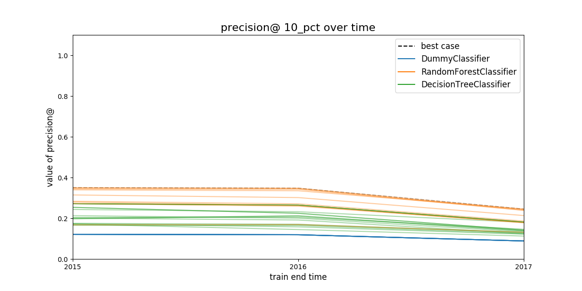Figure. Model group performance over time. In this case the metric show is precision@10%. The black dashed line represents the (theoretical) system's performance if we select the best performant model in a every evaluation date. The colored lines represents different model groups. All the model groups that share an algorithm will be colored the same.

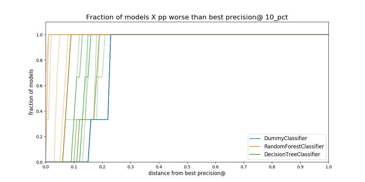Figure. Proportion of **all* the models in a model group that are separated from the best model. The distance is measured in percentual points, i.e. How much less precision at 10 percent of the population compared to the best model in that date.*

Selecting the best rule or strategy for choosing model groups#

In this phase of the audition, you will see what will happen in the next time if you choose your model group with an specific strategy or rule.

You then, can calculate the regret. Regret is defined as the difference between the performance of the best model evaluated on the "next time" and the performance of the model selected by a particular rule.

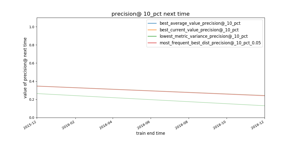Figure. Given a strategy for selecting model groups (in the plot 4 are shown), What will be the performace of the model group chosen by that strategy in the next evaluation date?

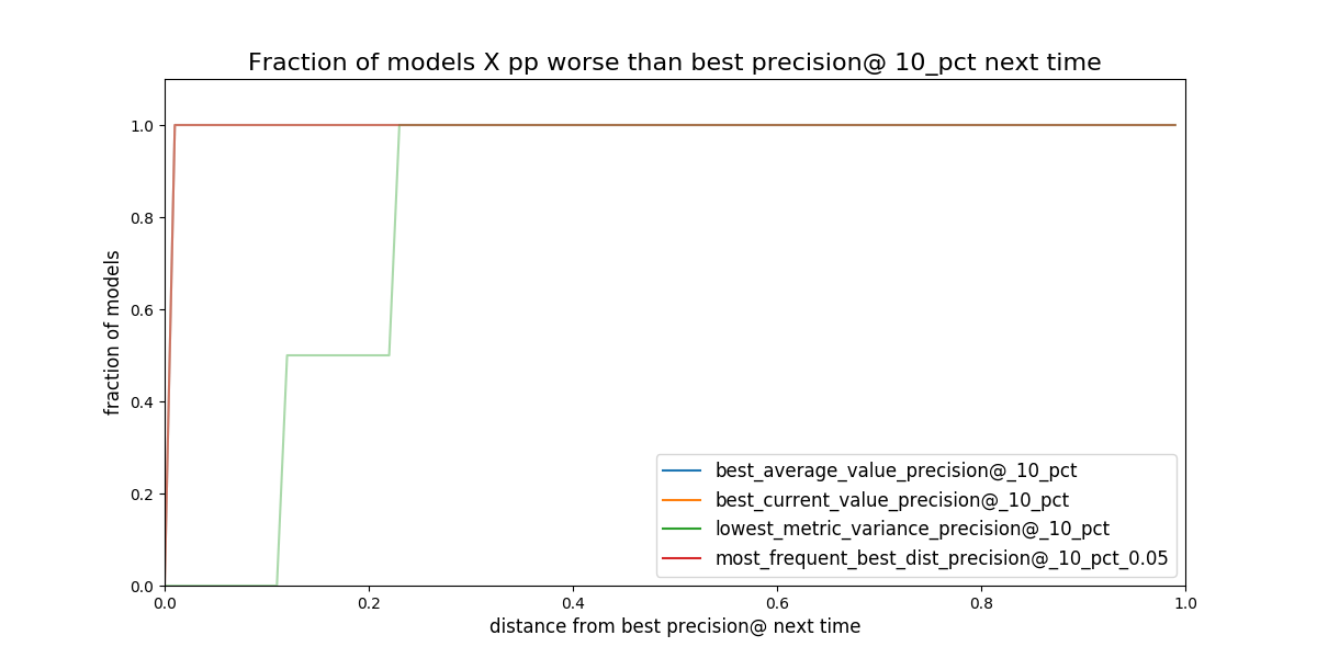Figure. Given a strategy for selecting model groups (in the plot 4 are shown). What will be the distance (*regret) to the best theoretical model in the following evaluation date.*

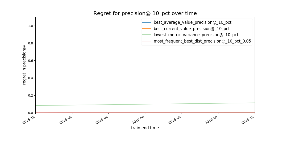Figure. Expected regret for the strategies. The less the better.

It seems that the worst strategy (the one with the bigger “regret”) for selecting a model_group is lowest_metric_variance_precision. The other three seem almost indistinguishable. We will dig in using Postmodeling. And afterwards instead of using the feature importance to characterize the facilities, we will explore how the model is splitting the facilities using crosstabs.

As before, the best 3 model groups per strategy will be stored in the file /triage/audition/eis/results_model_group_ids.json

{
    "most_frequent_best_dist_precision@_10_pct_0.05": [
        15,
        16,
        17,
        9,
        18
    ],
    "lowest_metric_variance_precision@_10_pct": [
        2,
        5,
        19,
        11,
        6
    ],
    "best_average_value_precision@_10_pct": [
        15,
        16,
        17,
        18,
        9
    ],
    "best_current_value_precision@_10_pct": [
        9,
        16,
        15,
        17,
        18
    ]
}

Postmodeling: Inspecting the best models closely#

Given that almost all the strategies perform well, we will change the parameter model_group_id in the postmodeling's configuration file and we will use the complete set of model groups selected by audition:

# Postmodeling Configuration File

  project_path: '/triage' # Project path defined in triage with matrices and models
  audition_output_path: '/triage/audition/eis/results_model_group_ids.json'

  thresholds: # Thresholds for2 defining positive predictions
        rank_abs: [50, 100, 250]
        rank_pct: [5, 10, 25]

  baseline_query: | # SQL query for defining a baseline for comparison in plots. It needs a metric and parameter
      select g.model_group_id,
             m.model_id,
             extract('year' from m.evaluation_end_time) as as_of_date_year,
             m.metric,
             m.parameter,
             m.stochastic_value,
             m.num_labeled_examples,
             m.num_labeled_above_threshold,
             m.num_positive_labels
       from test_results.evaluations m
       left join triage_metadata.models g
       using(model_id)
       where g.model_group_id = 20
             and metric = 'precision@'
             and parameter = '10_pct'

  max_depth_error_tree: 5 # For error trees, how depth the decision trees should go?
  n_features_plots: 10 # Number of features for importances
  figsize: [12, 12] # Default size for plots
  fontsize: 20 # Default fontsize for plots

Launch jupyter in bastion:

jupyter-notebook –-ip=0.0.0.0  --port=56406 --allow-root

And then in your browser location bar type: http://0.0.0.0:56406

Setup#

%matplotlib inline
import pandas as pd
import numpy as np
from collections import OrderedDict
from triage.component.postmodeling.contrast.utils.aux_funcs import create_pgconn, get_models_ids
from triage.component.catwalk.storage import ProjectStorage, ModelStorageEngine, MatrixStorageEngine
from triage.component.postmodeling.contrast.parameters import PostmodelParameters
from triage.component.postmodeling.contrast.model_evaluator import ModelEvaluator
from triage.component.postmodeling.contrast.model_group_evaluator import ModelGroupEvaluator

params = PostmodelParameters('../triage/eis_postmodeling_config.yaml')

engine = create_pgconn('database.yaml')

# Model group object (useful to compare across model_groups and models in time)
audited_models_class = ModelGroupEvaluator(tuple(params.model_group_id), engine)

Model groups#

Let’s start with the behavior in time of the selected model groups

audited_models_class.plot_prec_across_time(param_type='rank_pct',
                                           param=10,
                                           baseline=True,
                                           baseline_query=params.baseline_query,
                                           metric='precision@',
                                           figsize=params.figsize)

Every model selected by audition has a very similar performance across time, and they are ~2.5 times above the baseline in precision@10%. We could also check the recall of the model groups.

audited_models_class.plot_prec_across_time(param_type='rank_pct',
                                           param=10,
                                           metric='recall@',
                                           figsize=params.figsize)

That behavior is similar for the recall@10%, except for the model group 69

audited_models_class.plot_jaccard_preds(param_type='rank_pct',
                                        param=10,
                                        temporal_comparison=True)

There are a high jaccard similarity between some model groups across time. This could be an indicator that they are so similar that you can choose any and it won’t matter.

Going deeper with a model#

We will choose the model group 64 as the winner.

select
    mg.model_group_id,
    mg.model_type,
    mg.hyperparameters,
    array_agg(model_id order by train_end_time) as models
from
    triage_metadata.model_groups as mg
    inner join
    triage_metadata.models
    using (model_group_id)
where model_group_id = 76
group by 1,2,3

model_group_id	model_type	hyperparameters	models
64	sklearn.ensemble.RandomForestClassifier	{"criterion": "gini", "max_features": "sqrt", "n_estimators": 500, "min_samples_leaf": 1, "min_samples_split": 50}	{190,208,226}

But before going to production and start making predictions in unseen data, let’s see what the particular models are doing. Postmodeling created a ModelEvaluator (similar to the ModelGroupEvaluator) to do this exploration:

models_76 = { f'{model}': ModelEvaluator(76, model, engine) for model in [198,216,234] }

In this tutorial, we will just show some parts of the analysis in the most recent model, but feel free of exploring the behavior of all the models in this model group, and check if you can detect any pattern.

Feature importances

models_76['234'].plot_feature_importances(path=params.project_path,
                                          n_features_plots=params.n_features_plots,
                                          figsize=params.figsize)

models_76['234'].plot_feature_group_aggregate_importances()

Crosstabs: How are the entities classified?#

Model interpretation is a huge topic nowadays, the most obvious path is using the features importance from the model. This could be useful, but we could do a lot better.

Triage uses crosstabs as a different approach that complements the list of features importance. crosstabs will run statistical tests to compare the predicted positive and the predicted false facilities in each feature.

output:
  schema: 'test_results'
  table: 'eis_crosstabs'

thresholds:
    rank_abs: [50]
    rank_pct: [5]

#(optional): a list of entity_ids to subset on the crosstabs analysis
entity_id_list: []

models_list_query: "select unnest(ARRAY[226]) :: int as model_id"

as_of_dates_query: "select generate_series('2017-12-01'::date, '2018-09-01'::date, interval '1month')  as as_of_date"

#don't change this query unless strictly necessary. It is just validating pairs of (model_id,as_of_date)
#it is just a join with distinct (model_id, as_of_date) in a predictions table
models_dates_join_query: |
  select model_id,
  as_of_date
  from models_list_query as m
  cross join as_of_dates_query a join (select distinct model_id, as_of_date from test_results.predictions) as p
  using (model_id, as_of_date)

#features_query must join models_dates_join_query with 1 or more features table using as_of_date
features_query: |
  select m.model_id, m.as_of_date, f4.entity_id, f4.results_entity_id_1month_result_fail_avg, f4.results_entity_id_3month_result_fail_avg, f4.results_entity_id_6month_result_fail_avg,
  f2.inspection_types_entity_id_1month_type_canvass_sum, f3.risks_entity_id_1month_risk_high_sum, f4.results_entity_id_6month_result_pass_avg,
  f3.risks_entity_id_all_risk_high_sum, f2.inspection_types_entity_id_3month_type_canvass_sum, f4.results_entity_id_6month_result_pass_sum,
  f2.inspection_types_entity_id_all_type_canvass_sum
  from features.inspection_types_aggregation_imputed as f2
  inner join features.risks_aggregation_imputed as f3 using (entity_id, as_of_date)
  inner join features.results_aggregation_imputed as f4 using (entity_id, as_of_date)
  inner join models_dates_join_query as m using (as_of_date)

#the predictions query must return model_id, as_of_date, entity_id, score, label_value, rank_abs and rank_pct
#it must join models_dates_join_query using both model_id and as_of_date
predictions_query: |
  select model_id,
      as_of_date,
      entity_id,
      score,
      label_value,
      coalesce(rank_abs_no_ties, row_number() over (partition by (model_id, as_of_date) order by score desc)) as rank_abs,
      coalesce(rank_pct_no_ties*100, ntile(100) over (partition by (model_id, as_of_date) order by score desc)) as rank_pct
      from test_results.predictions
      join models_dates_join_query using(model_id, as_of_date)
      where model_id in (select model_id from models_list_query)
      and as_of_date in (select as_of_date from as_of_dates_query)

triage --tb crosstabs /triage/eis_crosstabs_config.yaml

When it finishes, you could explore the table with the following code:

with significant_features as (
select
    feature_column,
    as_of_date,
    threshold_unit
from
    test_results.eis_crosstabs
where
    metric = 'ttest_p'
    and
    value < 0.05 and as_of_date = '2018-09-01'
    )

select
    distinct
    model_id,
    as_of_date::date as as_of_date,
    format('%s %s', threshold_value, t1.threshold_unit) as threshold,
    feature_column,
    value as "ratio PP / PN"
from
    test_results.eis_crosstabs as t1
    inner join
    significant_features as t2 using(feature_column, as_of_date)
where
    metric = 'ratio_predicted_positive_over_predicted_negative'
    and
    t1.threshold_unit = 'pct'
order by value desc

model_id	as_of_date	threshold	feature_column	ratio PP / PN
226	2018-09-01	5 pct	results_entity_id_1month_result_fail_avg	11.7306052855925
226	2018-09-01	5 pct	results_entity_id_3month_result_fail_avg	3.49082798996376
226	2018-09-01	5 pct	results_entity_id_6month_result_fail_avg	1.27344759545161
226	2018-09-01	5 pct	risks_zip_code_1month_risk_high_sum	1.17488357227451
226	2018-09-01	5 pct	inspection_types_entity_id_all_type_canvass_sum	0.946432281075976
226	2018-09-01	5 pct	inspection_types_zip_code_3month_type_canvass_sum	0.888940127100436
226	2018-09-01	5 pct	results_entity_id_6month_result_pass_sum	0.041806916457784
226	2018-09-01	5 pct	results_entity_id_6month_result_pass_avg	0.0232523724927717

This table represents the ratio between the predicted positives at the top 5% and predicted negatives (the rest). For example, you can see that in PP are eleven times more inspected if they have a failed inspection in the last month, 3.5 times more if they have a failed inspection in the previous 3 months, etc.

Where to go from here#

Ready to get started with your own data? Check out the suggested project workflow for some tips about how to iterate and tune the pipeline for your project.

Want to work through another example? Take a look at our resource prioritization case study