Resource prioritization systems: Chicago food inspections#

Before continue, Did you…?

This case study, part of the dirtyduck tutorial, assumes that you already setup the tutorial’s infrastructure and load the dataset.

If you didn’t setup the infrastructure go here,
If you didn't load the data, you can do it very quickly or you can follow all the steps and explanations about the data.

Problem description#

We want to generate a list of facilities that will have a critical or serious food violation if inspected.

The scenario is the following: you work for the City of Chicago and you have limited food inspectors, so you try to prioritize them to focus on the highest-risk facilities. So you will use the data to answer the next question:

Which $X$ facilities are most likely to fail a food inspection in the following $Y$ period of time?

A more technical way of writing the question is: What is the probability distribution of facilities that are at risk of fail a food inspection if they are inspected in the following period of time?¹

If you want to focus on major violations only, you can do that too:

Which $X$ facilities are most likely to have a critical or serious violation in the following $Y$ period of time?

This situation is very common in governmental agencies that provide social services: they need to prioritize their resources and use them in the facilities that are most likely to have problems

We will use machine learning to accomplish this. This means that we will use historical data to train our models, and we will use temporal cross validation to test the performance of them.

For the resource prioritization problems there are commonly two problems with the data: (a) bias and (b) incompleteness.

First, note that our data have bias: We only have data on facilities that were inspected. That means that our data set contains information about the probability of have a violation ( $V$ ) given that the facility was inspected ( $I$ ), $P(V|I)$ . But the probability that we try to find is $P(V)$ .

A different problem that our data set could have is if our dataset contains all the facilities in Chicago, i.e. if our entities table represents the Universe of facilities. There are almost 40,000 entities in our database. We could make the case that every facility in Chicago is in the database, since every facility that opens will be subject to an inspection. We will assume that all the facilities are in our data.

What do you want to predict?#

We are interested in two different outcomes:

Which facilities are likely to fail an inspection?

The outcome takes a 1 if the inspection had at least one result = 'fail' and a 0 otherwise.

Which facilities fail an inspection with a major violation?

Critical violations are coded between 1-14, serious violations between 15-29, everything above 30 is assumed to be a minor violation. The label takes a 1 if the inspection had at least one result = 'fail' and a violation between 1 and 29, and a 0 otherwise.

I want to learn more about the data

Check the Data preparation section!

Data Changes

On 7/1/2018 the Chicago Department of Public Health’s Food Protection unit changed the definition of violations. The changes don’t affect structurally the dataset (e.g. how the violations are inputted to the database), but the redefinition will change the distribution and interpretation of the violation codes. See here.

We can extract the severity of the violation using the following code:

select
    event_id,
    entity_id,
    date,
    result,
    array_agg(distinct obj ->>'severity') as violations_severity,
    (result = 'fail') as failed,
    coalesce(
    (result = 'fail' and
        ('serious' = ANY(array_agg(obj ->> 'severity')) or 'critical' = ANY(array_agg(obj ->> 'severity')))
        ), false
    ) as failed_major_violation
from
    (
    select
        event_id,
        entity_id,
        date,
        result,
        jsonb_array_elements(violations::jsonb) as obj
    from
        semantic.events
        limit 20
        ) as t1
group by
    entity_id, event_id, date, result
order by
   date desc;

event_id	entity_id	date	result	violations_severity	failed	failed_major_violation
1770568	30841	2016-05-11	pass	{minor}	f	f
1763967	30841	2016-05-03	fail	{critical,minor,serious}	t	t
1434534	21337	2014-04-03	pass	{NULL}	f	f
1343315	22053	2013-06-06	fail	{minor,serious}	t	t
1235707	21337	2013-03-27	pass	{NULL}	f	f
537439	13458	2011-06-10	fail	{NULL}	t	f
569377	5570	2011-06-01	pass	{NULL}	f	f

The outcome will be used by triage to generate the labels (once that we define a time span of interest). The following image tries to show the meaning of the outcomes for the inspection failed problem definition.

Figure. The image shows three facilities (blue, red and orange) and, next to each, a temporal line with 6 days (0-5). Each dot represents an inspection. Color is the **outcome* of the inspection. Green means the facility passed the inspection, and red means it failed. Each facility in the image had two inspections, but only the facility in the middle passed both.*

Modeling Using Machine Learning#

It is time to put these steps together. All the coding is complete (triage dev team did that for us); we just need to modify the triage experiment’s configuration file.

Defining a baseline#

As a first step, lets do an experiment that defines our baseline. The rationale of this is that the knowing the baseline will allow us to verify if our Machine Learning model is better than the baseline. The baseline in our example will be a random selection of facilities². This is implemented as a DummyClassifier in scikit-learn. Another advantage of starting with the baseline, is that is very fast to train (DummyClassifier is not computationally expensive) , so it will help us to verify that the experiment configuration is correct without waiting for a long time.

Experiment description file

You could check the meaning about experiment description files (or configuration files) in A deeper look into triage.

We need to write the experiment config file for that. Let's break it down and explain their sections.

The config file for this first experiment is located in inspections_baseline.yaml.

The first lines of the experiment config file specify the config-file version (v8 at the moment of writing this tutorial), a comment (model_comment, which will end up as a value in the triage_metadata.models table), and a list of user-defined metadata (user_metadata) that can help to identify the resulting model groups. For this example, if you run experiments that share a temporal configuration but that use different label definitions (say, labeling inspections with any violation as positive versus only labeling inspections with major violations as positive), you can use the user metadata keys to indicate that the matrices from these experiments have different labeling criteria. The matrices from the two experiments will have different filenames (and should not be overwritten or incorrectly used), and if you add the label_definition key to the model_group_keys, models made on different label definitions will belong to different model groups.

config_version: 'v8'

model_comment: 'inspections: baseline'
random_seed: 23895478

user_metadata:
    label_definition: 'failed'
    file_name: 'inspections_baseline.yaml'
    experiment_type: 'inspections prioritization'
    description: |
      Baseline calculation
    purpose: 'baseline'
    org: 'DSaPP'
    team: 'Tutorial'
    author: 'Your name here'
    etl_date: '2019-05-07'

model_group_keys:
  - 'class_path'
  - 'parameters'
  - 'feature_names'
  - 'feature_groups'
  - 'cohort_name'
  - 'state'
  - 'label_name'
  - 'label_timespan'
  - 'training_as_of_date_frequency'
  - 'max_training_history'
  - 'label_definition'
  - 'experiment_type'
  - 'org'
  - 'team'
  - 'author'
  - 'etl_date'

Note

Obviously, change 'Your name here' for your name (if you like)

Next comes the temporal configuration section. The first four parameters are related to the availability of data: How much data you have for feature creation? How much data you have for label generation?

Data Changes

On 7/1/2018 the Chicago Department of Public Health’s Food Protection unit changed the definition of violations. The changes don’t affect structurally the dataset (e.g. how the violations are inputted to the database), but the redefinition will change the distribution and interpretation of the violation codes. See here.

The next parameters are related to the training intervals:

How frequently to retrain models? (model_update_frequency)
How many rows per entity in the train matrices? (training_as_of_date_frequencies)
How much time is covered by labels in the training matrices? (training_label_timespans)

The remaining elements are related to the testing matrices. For inspections, you can choose them as follows:

test_as_of_date_frequencies is planning/scheduling frequency
test_durations how far ahead do you schedule inspections?
test_label_timespan is equal to test_durations

Let's assume that we need to do rounds of inspections every 6 months (test_as_of_date_frequencies = 6month) and we need to complete that round in exactly in that time (i.e. 6 months) (test_durations = test_label_timespan = 6month).

We will assume that the data is more or less stable³, at least for now, so model_update_frequency = 6month.

temporal_config:
    feature_start_time: '2010-01-04'
    feature_end_time: '2018-06-01'
    label_start_time: '2015-01-01'
    label_end_time: '2018-06-01'

    model_update_frequency: '6month'
    training_label_timespans: ['6month']
    training_as_of_date_frequencies: '6month'

    test_durations: '0d'
    test_label_timespans: ['6month']
    test_as_of_date_frequencies: '6month'

    max_training_histories: '5y'

We can visualize the time splitting using the function show-timechop (See A deeper look into triage for more information)

# Remember to run this in bastion  NOT in your laptop shell!
triage experiment experiments/inspections_baseline.yaml --show-timechop

Figure. Temporal blocks for the inspections baseline experiment

We need to specify our labels. For this first experiment we will use the label failed, using the same query from the simple_skeleton_experiment.yaml

label_config:
  query: |
    select
    entity_id,
    bool_or(result = 'fail')::integer as outcome
    from semantic.events
    where '{as_of_date}'::timestamp <= date
    and date < '{as_of_date}'::timestamp + interval '{label_timespan}'
    group by entity_id
  name: 'failed_inspections'

It should be obvious, but let's state it anyway: We are only training in facilities that were inspected, but we will test our model in all the facilities in our cohort⁴. So, in the train matrices we will have only 0 and 1 as possible labels, but in the test matrices we will found 0, 1 and NULL.

I want to learn more about this…

In the section regarding to Early Warning Systems we will learn how to incorporate all the facilities of the cohort in the train matrices.

We just want to include active facilities in our matrices, so we tell triage to take that in account:

cohort_config:
  query: |
    select e.entity_id
    from semantic.entities as e
    where
    daterange(start_time, end_time, '[]') @> '{as_of_date}'::date
  name: 'active_facilities'

Triage will generate the features for us, but we need to tell it which features we want in the section feature_aggregations. Here, each entry describes a collate.SpacetimeAggregation object and the arguments needed to create it⁵. For this experiment, we will use only one feature (number of inspections). DummyClassifier don't use any feature to do the "prediction", so we won't expend compute cycles doing the feature/matrix creation:

feature_aggregations:
  -
    prefix: 'inspections'
    from_obj: 'semantic.events'
    knowledge_date_column: 'date'

    aggregates_imputation:
      count:
        type: 'zero_noflag'

    aggregates:
       -
        quantity:
          total: "*"
        metrics:
          - 'count'

    intervals: ['all']

feature_group_definition:
   prefix:
     - 'inspections'

feature_group_strategies: ['all']

If we observe the image generated from the temporal_config section, each particular date is the beginning of the rectangles that describes the rows in the matrix. In that date (as_of_date in timechop parlance) we will calculate the feature, and we will repeat that for every other rectangle in that image.

Now, let's discuss how we will specify the models to try (remember that the model is specified by the algorithm, the hyperparameters, and the subset of features to use). In triage you need to specify in the grid_config section a list of machine learning algorithms that you want to train and a list of hyperparameters. You can use any algorithm that you want; the only requirement is that it respects the sklearn API.

grid_config:
    'sklearn.dummy.DummyClassifier':
        strategy: [uniform]

Finally, we should define wich metrics we care about for evaluating our model. Here we will concentrate only in precision and recall at an specific value $k$ ⁶.

In this setting $k$ represents the resource’s constraint: It is the number of inspections that the city could do in a month given all the inspectors available.

scoring:
    testing_metric_groups:
        -
          metrics: [precision@, recall@, 'false negatives@', 'false positives@', 'true positives@', 'true negatives@']
          thresholds:
            percentiles: [1.0, 2.0, 3.0, 4.0, 5.0, 10, 15, 20, 25, 30, 35, 40, 45, 50, 55, 60, 65, 70, 75, 80, 85, 90, 95, 100]
            top_n: [1, 5, 10, 25, 50, 100, 250, 500, 1000]
        -
          metrics: [auc, accuracy]

    training_metric_groups:
      -
        metrics: [auc, accuracy]
      -
        metrics: [precision@, recall@]
        thresholds:
          percentiles: [1.0, 2.0, 3.0, 4.0, 5.0, 10, 15, 20, 25, 30, 35, 40, 45, 50, 55, 60, 65, 70, 75, 80, 85, 90, 95, 100]
          top_n: [1, 5, 10, 25, 50, 100, 250, 500, 1000]

You should be warned that precision and recall at $k$ in this setting is kind of ill-defined (because you will end with a lot of NULL labels, remember, only a few of facilities are inspected in each period)⁷.

We will want a list of facilities to be inspected. The length of our list is constrained by our inspection resources, i.e. the answer to the question How many facilities can I inspect in a month? In this experiment we are assuming that the maximum capacity is 10% but we are evaluating for a larger space of possibilities (see top_n, percentiles above).

The execution of the experiments can take a long time, so it is a good practice to validate the configuration file before running the model. You don't want to wait for hours (or days) and then discover that something went wrong.

# Remember to run this in bastion  NOT in your laptop shell!
triage experiment experiments/inspections_baseline.yaml  --validate-only

If everything was ok, you should see an Experiment validation ran to completion with no errors.

You can execute the experiment as⁸

# Remember to run this in bastion  NOT in your laptop shell!
time triage experiment experiments/inspections_baseline.yaml

Protip

We are including the command time in order to get the total running time of the experiment. You can remove it, if you like.

Don’t be scared!

This will print a lot of output! It is not an error!

We can query the table experiments to see the quantity of work that triage needs to do

select
    substring(experiment_hash, 1,4) as experiment,
    config -> 'user_metadata' ->> 'description'  as description,
    total_features,
    matrices_needed,
    models_needed
from triage_metadata.experiments;

experiment	description	total_features	matrices_needed	models_needed
e912	"Baseline calculation\n"	1	10	5

If everything is correct, triage will create 10 matrices (5 for training, 5 for testing) in triage/matrices and every matrix will be represented by two files, one with the metadata of the matrix (a yaml file) and one with the actual matrix (the gz file).

# We will use some bash magic

ls matrices | awk -F . '{print $NF}' | sort | uniq -c

Triage also will store 5 trained models in triage/trained_models:

ls trained_models | wc -l

And it will populate the results schema in the database. As mentioned, we will get 1 model groups:

select
    model_group_id,
    model_type,
    hyperparameters
from
    triage_metadata.model_groups
where
    model_config ->> 'experiment_type' ~ 'inspection'

model_group_id	model_type	hyperparameters
1	sklearn.dummy.DummyClassifier	{"strategy": "prior"}

And 5 models:

select
    model_group_id,
    array_agg(model_id) as models,
    array_agg(train_end_time::date) as train_end_times
from
    triage_metadata.models
where
    model_comment ~ 'inspection'
group by
    model_group_id
order by
    model_group_id;

model_group_id	models	train_end_times
1	{1,2,3,4,5}	{2015-12-01,2016-06-01,2016-12-01,2017-06-01,2017-12-01}

From that last query, you should note that the order in which triage trains the models is from oldest to newest train_end_time and model_group , also in ascending order. It will not go to the next block until all the models groups are trained.

You can check on which matrix each models were trained:

select
    model_group_id,
    model_id, train_end_time::date,
    substring(model_hash,1,5) as model_hash,
    substring(train_matrix_uuid,1,5) as train_matrix_uuid,
    ma.num_observations as observations,
    ma.lookback_duration as feature_lookback_duration,  ma.feature_start_time
from
    triage_metadata.models as mo
    join
    triage_metadata.matrices as ma
    on train_matrix_uuid = matrix_uuid
where
    mo.model_comment ~ 'inspection'
order by
    model_group_id,
    train_end_time asc;

model_group_id	model_id	train_end_time	model_hash	train_matrix_uuid	observations	feature_lookback_duration	feature_start_time
1	1	2015-12-01	743a6	1c266	5790	5 years	2010-01-04 00:00:00
1	2	2016-06-01	5b656	755c6	11502	5 years	2010-01-04 00:00:00
1	3	2016-12-01	5c170	2aea8	17832	5 years	2010-01-04 00:00:00
1	4	2017-06-01	55c3e	3efdc	23503	5 years	2010-01-04 00:00:00
1	5	2017-12-01	ac993	a3762	29112	5 years	2010-01-04 00:00:00

Each model was trained with the matrix indicated in the column train_matrix_uuid. This uuid is the file name of the stored matrix. The model itself was stored under the file named with the model_hash.

If you want to see in which matrix the model was tested you need to run the following query

select distinct
    model_id,
    model_group_id, train_end_time::date,
    substring(model_hash,1,5) as model_hash,
    substring(ev.matrix_uuid,1,5) as test_matrix_uuid,
    ma.num_observations as observations
from
    triage_metadata.models as mo
    join
    test_results.evaluations as ev using (model_id)
    join
    triage_metadata.matrices as ma on ev.matrix_uuid = ma.matrix_uuid
where
    mo.model_comment ~ 'inspection'
order by
    model_group_id, train_end_time asc;

model_id	model_group_id	train_end_time	model_hash	test_matrix_uuid	observations
1	1	2015-12-01	743a6	4a0ea	18719
2	1	2016-06-01	5b656	f908e	19117
3	1	2016-12-01	5c170	00a88	19354
4	1	2017-06-01	55c3e	8f3cf	19796
5	1	2017-12-01	ac993	417f0	20159

All the models were stored in /triage/trained_models/{model_hash} using the standard serialization of sklearn models. Every model was trained with the matrix train_matrix_uuid stored in the directory /triage/matrices.

What's the performance of this model groups?

\set k 0.10    -- This defines a variable, "k = 0.10"

select distinct
    model_group_id,
    model_id,
    ma.feature_start_time::date,
    train_end_time::date,
    ev.evaluation_start_time::date,
    ev.evaluation_end_time::date,
    to_char(ma.num_observations, '999,999') as observations,
    to_char(ev.num_labeled_examples, '999,999') as "total labeled examples",
    to_char(ev.num_positive_labels, '999,999') as "total positive labels",
    to_char(ev.num_labeled_above_threshold, '999,999') as "labeled examples@k%",
    to_char(:k * ma.num_observations, '999,999') as "predicted positive (PP)",
    ARRAY[to_char(ev.best_value * ev.num_labeled_above_threshold,'999,999'),
          to_char(ev.worst_value * ev.num_labeled_above_threshold,'999,999'),
          to_char(ev.stochastic_value * ev.num_labeled_above_threshold, '999,999')]
    as "true positive (TP)@k% (best,worst,stochastic)",
    ARRAY[ to_char(ev.best_value, '0.999'), to_char(ev.worst_value, '0.999'),
    to_char(ev.stochastic_value, '0.999')]  as "precision@k% (best,worst,stochastic)",
    to_char(ev.num_positive_labels*1.0 / ev.num_labeled_examples, '0.999') as baserate,
    :k * 100 as "k%"
from
    triage_metadata.models as mo
    join
    test_results.evaluations as ev using (model_id)
    join
    triage_metadata.matrices as ma on ev.matrix_uuid = ma.matrix_uuid
where
    ev.metric || ev.parameter = 'precision@15_pct'
    and
    mo.model_comment ~ 'inspection'
order by
    model_id, train_end_time asc;
order by
    model_id, train_end_time asc;

model_group_id	model_id	feature_start_time	train_end_time	evaluation_start_time	evaluation_end_time	observations	total labeled examples	total positive labels	predicted positive (PP)	true positive (TP)@k% (best,worst,stochastic)	precision@k% (best,worst,stochastic)	baserate	k%
21	121	2010-01-04	2015-12-01	2015-12-01	2015-12-01	18,719	5,712	1,509	2,808	{" 0"," 0"," 0"}	{" 0.000"," 0.000"," 0.000"}	0.264	15.00
21	122	2010-01-04	2016-06-01	2016-06-01	2016-06-01	19,117	6,330	1,742	2,868	{" 0"," 0"," 0"}	{" 0.000"," 0.000"," 0.000"}	0.275	15.00
21	123	2010-01-04	2016-12-01	2016-12-01	2016-12-01	19,354	5,671	1,494	2,903	{" 0"," 0"," 0"}	{" 0.000"," 0.000"," 0.000"}	0.263	15.00
21	124	2010-01-04	2017-06-01	2017-06-01	2017-06-01	19,796	5,609	1,474	2,969	{" 0"," 0"," 0"}	{" 0.000"," 0.000"," 0.000"}	0.263	15.00
21	125	2010-01-04	2017-12-01	2017-12-01	2017-12-01	20,159	4,729	1,260	3,024	{" 0"," 0"," 0"}	{" 0.000"," 0.000"," 0.000"}	0.266	15.00

The columns num_labeled_examples, num_labeled_above_threshold, num_positive_labels represent the number of selected entities on the prediction date that are labeled, the number of entities with a positive label above the threshold, and the number of entities with positive labels among all the labeled entities respectively.

We added some extra columns: baserate, predicted positive (PP) and true positive (TP). Baserate represents the proportion of the all the facilities that were inspected that failed the inspection, i.e. $P(V|I)$ . The PP and TP are approximate since it were calculated using the value of $k$ or the precision value. But you could get the exact value of those from the test_results.predictions table.

Also note that in the precision@k% column we are showing three numbers: best, worst, stochastic.

They try to answer the question How do you break ties in the prediction score? This is important because it will affect the calculation of your metrics. The Triage proposed solution to this is calculate the metric in the best case scenario (score descending, all the true labels are at the top), and then do it in the worst case scenario (score descending, all the true labels are at the bottom) and then calculate the metric several times ( $n=30$ ) with the labels randomly shuffled (a.k.a. stochastic scenario), so you get the mean metric, plus some confidence intervals.

This problem is not specific of an inspection problem, is more related to simple models like a shallow Decision Tree or a Dummy Classifier when score ties likely will occur.

Note how in this model, the stochastic value is close to the baserate, since we are selecting at random using the prior.

Check this!

Note that the baserate should be equal to the precision@100%, if is not there is something wrong …

Creating a simple experiment#

We will try two of the simplest machine learning algorithms: a Decision Tree Classifier (DT) and a Scaled Logistic Regression (SLR)¹² as a second experiment. The rationale of this is that the DT is very fast to train (so it will help us to verify that the experiment configuration is correct without waiting for a long time) and it helps you to understand the structure of your data.

The config file for this first experiment is located in /triage/experiments/inspections_dt.yaml

Note that we don't modify the temporal_config section neither the feature_aggregations, cohort_config or label_config. Triage is smart enough to use the previous tables and matrices instead of generating them from scratch.

config_version: 'v8'

model_comment: 'inspections: basic ML'

user_metadata:
  label_definition: 'failed'
  experiment_type: 'inspections prioritization'
  file_name: 'inspections_dt.yaml'
  description: |
    DT and SLR
  purpose: 'data mining'
  org: 'DSaPP'
  team: 'Tutorial'
  author: 'Your name here'
  etl_date: '2019-02-21'

Note that we don't modify the temporal_config section neither the cohort_config or label_config. Triage is smart enough to use the previous tables and matrices instead of generating them from scratch.

For this experiment, we will add the following features:

Number of different types of inspections the facility had in the last year (calculated for an as-of-date).
Number of different types of inspections that happened in the zip code in the last year from a particular day.
Number of inspections
Number/proportion of inspections by result type
Number/proportion of times that a facility was classify with particular risk level

In all of them we will do the aggregation in the last month, 3 months, 6 months, 1 year and historically. Remember that all this refers to events in the past, i.e. How many times the facility was marked with high risk in the previous 3 Months?, What is the proportion of failed inspections in the previous year?

feature_aggregations:
  -
    prefix: 'inspections'
    from_obj: 'semantic.events'
    knowledge_date_column: 'date'

    aggregates_imputation:
      count:
        type: 'zero_noflag'

    aggregates:
      -
        quantity:
          total: "*"
        metrics:
          - 'count'

    intervals: ['1month', '3month', '6month', '1y', 'all']

  -
    prefix: 'risks'
    from_obj: 'semantic.events'
    knowledge_date_column: 'date'

    categoricals_imputation:
      sum:
        type: 'zero'
      avg:
        type: 'zero'

    categoricals:
      -
        column: 'risk'
        choices: ['low', 'medium', 'high']
        metrics:
          - 'sum'
          - 'avg'

    intervals: ['1month', '3month', '6month', '1y', 'all']

  -
    prefix: 'results'
    from_obj: 'semantic.events'
    knowledge_date_column: 'date'

    categoricals_imputation:
      all:
        type: 'zero'

    categoricals:
      -
        column: 'result'
        choice_query: 'select distinct result from semantic.events'
        metrics:
          - 'sum'
          - 'avg'

    intervals: ['1month', '3month', '6month', '1y', 'all']

  -
    prefix: 'inspection_types'
    from_obj: 'semantic.events'
    knowledge_date_column: 'date'

    categoricals_imputation:
      sum:
        type: 'zero_noflag'

    categoricals:
      -
        column: 'type'
        choice_query: 'select distinct type from semantic.events where type is not null'
        metrics:
          - 'sum'

    intervals: ['1month', '3month', '6month', '1y', 'all']

And as stated, we will train some Decision Trees, in particular we are interested in some shallow trees, and in a full grown tree. These trees will show you the structure of your data. We also will train some Scaled Logistic Regression, this will show us how "linear" is the data (or how the assumptions of the Logistic Regression holds in this data)

grid_config:
  'sklearn.tree.DecisionTreeClassifier':
        criterion: ['gini']
        max_features: ['sqrt']
        max_depth: [1, 2, 5,~]
        min_samples_split: [2,10,50]

  'triage.component.catwalk.estimators.classifiers.ScaledLogisticRegression':
        penalty: ['l1','l2']
        C: [0.000001, 0.0001, 0.01,  1.0]

About yaml and sklearn

Some of the parameters in sklearn are None. If you want to try those you need to indicate it with yaml's null or ~ keyword.

Besides the algorithm and the hyperparameters, you should specify which subset of features use. First, in the section feature_group_definition you specify how to group the features (you can use the table name or the prefix from the section feature_aggregation) and then a strategy for choosing the subsets: all (all the subsets at once), leave-one-out (try all the subsets except one, do that for all the combinations), or leave-one-in (just try subset at the time).

feature_group_definition:
   prefix:
     - 'inspections'
     - 'results'
     - 'risks'
     - 'inspection_types'

feature_group_strategies: ['all']

Finally we will leave the scoring section as before.

In this experiment we will end with 6 model groups (number of algorithms [1] $\times$ number of hyperparameter combinations [2 $\times$ 3 = 5] $\times$ number of feature groups strategies [1]]). Also, we will create 18 models (3 per model group) given that we have 3 temporal blocks (one model per temporal group).

Before running the experiment, remember to validate that the configuration is correct:

# Remember to run this in bastion  NOT in your laptop shell!
triage experiment experiments/inspections_dt.yaml  --validate-only

and check the temporal cross validation:

# Remember to run this in bastion  NOT in your laptop shell!
triage experiment experiments/inspections_dt.yaml --show-timechop

Temporal blocks for inspections experiment. The label is a failed inspection in the next year.

You can execute the experiment like this:

# Remember to run this in bastion  NOT in your laptop shell!
time triage experiment experiments/inspections_dt.yaml

Again, we can run the following sql to see which things triage needs to run:

select
    substring(experiment_hash, 1,4) as experiment,
    config -> 'user_metadata' ->> 'description'  as description,
    total_features,
    matrices_needed,
    models_needed
from triage_metadata.experiments;

experiment	description	total_features	matrices_needed	models_needed
e912	Baseline calculation	1	10	5
b535	DT and SLR	201	10	100

You can compare our two experiments and there are several differences, mainly in the order of magnitude. Like the number of features (1 vs 201) and models built (5 vs 100).

The After the experiment finishes, you will get 19 new model_groups (1 per combination in grid_config)

select
    model_group_id,
    model_type,
    hyperparameters
from
    triage_metadata.model_groups
where
    model_group_id not in (1);

model_group_id	model_type	hyperparameters
2	sklearn.tree.DecisionTreeClassifier	{"criterion": "gini", "max_depth": 1, "max_features": "sqrt", "min_samples_split": 2}
3	sklearn.tree.DecisionTreeClassifier	{"criterion": "gini", "max_depth": 1, "max_features": "sqrt", "min_samples_split": 10}
4	sklearn.tree.DecisionTreeClassifier	{"criterion": "gini", "max_depth": 1, "max_features": "sqrt", "min_samples_split": 50}
5	sklearn.tree.DecisionTreeClassifier	{"criterion": "gini", "max_depth": 2, "max_features": "sqrt", "min_samples_split": 2}
6	sklearn.tree.DecisionTreeClassifier	{"criterion": "gini", "max_depth": 2, "max_features": "sqrt", "min_samples_split": 10}
7	sklearn.tree.DecisionTreeClassifier	{"criterion": "gini", "max_depth": 2, "max_features": "sqrt", "min_samples_split": 50}
8	sklearn.tree.DecisionTreeClassifier	{"criterion": "gini", "max_depth": 5, "max_features": "sqrt", "min_samples_split": 2}
9	sklearn.tree.DecisionTreeClassifier	{"criterion": "gini", "max_depth": 5, "max_features": "sqrt", "min_samples_split": 10}
10	sklearn.tree.DecisionTreeClassifier	{"criterion": "gini", "max_depth": 5, "max_features": "sqrt", "min_samples_split": 50}
11	sklearn.tree.DecisionTreeClassifier	{"criterion": "gini", "max_depth": null, "max_features": "sqrt", "min_samples_split": 2}
12	sklearn.tree.DecisionTreeClassifier	{"criterion": "gini", "max_depth": null, "max_features": "sqrt", "min_samples_split": 10}
13	sklearn.tree.DecisionTreeClassifier	{"criterion": "gini", "max_depth": null, "max_features": "sqrt", "min_samples_split": 50}
14	triage.component.catwalk.estimators.classifiers.ScaledLogisticRegression	{"C": 0.000001, "penalty": "l1"}
15	triage.component.catwalk.estimators.classifiers.ScaledLogisticRegression	{"C": 0.000001, "penalty": "l2"}
16	triage.component.catwalk.estimators.classifiers.ScaledLogisticRegression	{"C": 0.0001, "penalty": "l1"}
17	triage.component.catwalk.estimators.classifiers.ScaledLogisticRegression	{"C": 0.0001, "penalty": "l2"}
18	triage.component.catwalk.estimators.classifiers.ScaledLogisticRegression	{"C": 0.01, "penalty": "l1"}
19	triage.component.catwalk.estimators.classifiers.ScaledLogisticRegression	{"C": 0.01, "penalty": "l2"}
20	triage.component.catwalk.estimators.classifiers.ScaledLogisticRegression	{"C": 1.0, "penalty": "l1"}
21	triage.component.catwalk.estimators.classifiers.ScaledLogisticRegression	{"C": 1.0, "penalty": "l2"}

and 100 models (as stated before)

select
    model_group_id,
    array_agg(model_id) as models,
    array_agg(train_end_time) as train_end_times
from
    triage_metadata.models
where
    model_group_id not in (1)
group by
    model_group_id
order by
    model_group_id;

model_group_id	models	train_end_times
2	{6,26,46,66,86}	{"2015-12-01 00:00:00","2016-06-01 00:00:00","2016-12-01 00:00:00","2017-06-01 00:00:00","2017-12-01 00:00:00"}
3	{7,27,47,67,87}	{"2015-12-01 00:00:00","2016-06-01 00:00:00","2016-12-01 00:00:00","2017-06-01 00:00:00","2017-12-01 00:00:00"}
4	{8,28,48,68,88}	{"2015-12-01 00:00:00","2016-06-01 00:00:00","2016-12-01 00:00:00","2017-06-01 00:00:00","2017-12-01 00:00:00"}
5	{9,29,49,69,89}	{"2015-12-01 00:00:00","2016-06-01 00:00:00","2016-12-01 00:00:00","2017-06-01 00:00:00","2017-12-01 00:00:00"}
6	{10,30,50,70,90}	{"2015-12-01 00:00:00","2016-06-01 00:00:00","2016-12-01 00:00:00","2017-06-01 00:00:00","2017-12-01 00:00:00"}
7	{11,31,51,71,91}	{"2015-12-01 00:00:00","2016-06-01 00:00:00","2016-12-01 00:00:00","2017-06-01 00:00:00","2017-12-01 00:00:00"}
8	{12,32,52,72,92}	{"2015-12-01 00:00:00","2016-06-01 00:00:00","2016-12-01 00:00:00","2017-06-01 00:00:00","2017-12-01 00:00:00"}
9	{13,33,53,73,93}	{"2015-12-01 00:00:00","2016-06-01 00:00:00","2016-12-01 00:00:00","2017-06-01 00:00:00","2017-12-01 00:00:00"}
10	{14,34,54,74,94}	{"2015-12-01 00:00:00","2016-06-01 00:00:00","2016-12-01 00:00:00","2017-06-01 00:00:00","2017-12-01 00:00:00"}
11	{15,35,55,75,95}	{"2015-12-01 00:00:00","2016-06-01 00:00:00","2016-12-01 00:00:00","2017-06-01 00:00:00","2017-12-01 00:00:00"}
12	{16,36,56,76,96}	{"2015-12-01 00:00:00","2016-06-01 00:00:00","2016-12-01 00:00:00","2017-06-01 00:00:00","2017-12-01 00:00:00"}
13	{17,37,57,77,97}	{"2015-12-01 00:00:00","2016-06-01 00:00:00","2016-12-01 00:00:00","2017-06-01 00:00:00","2017-12-01 00:00:00"}
14	{18,38,58,78,98}	{"2015-12-01 00:00:00","2016-06-01 00:00:00","2016-12-01 00:00:00","2017-06-01 00:00:00","2017-12-01 00:00:00"}
15	{19,39,59,79,99}	{"2015-12-01 00:00:00","2016-06-01 00:00:00","2016-12-01 00:00:00","2017-06-01 00:00:00","2017-12-01 00:00:00"}
16	{20,40,60,80,100}	{"2015-12-01 00:00:00","2016-06-01 00:00:00","2016-12-01 00:00:00","2017-06-01 00:00:00","2017-12-01 00:00:00"}
17	{21,41,61,81,101}	{"2015-12-01 00:00:00","2016-06-01 00:00:00","2016-12-01 00:00:00","2017-06-01 00:00:00","2017-12-01 00:00:00"}
18	{22,42,62,82,102}	{"2015-12-01 00:00:00","2016-06-01 00:00:00","2016-12-01 00:00:00","2017-06-01 00:00:00","2017-12-01 00:00:00"}
19	{23,43,63,83,103}	{"2015-12-01 00:00:00","2016-06-01 00:00:00","2016-12-01 00:00:00","2017-06-01 00:00:00","2017-12-01 00:00:00"}
20	{24,44,64,84,104}	{"2015-12-01 00:00:00","2016-06-01 00:00:00","2016-12-01 00:00:00","2017-06-01 00:00:00","2017-12-01 00:00:00"}
21	{25,45,65,85,105}	{"2015-12-01 00:00:00","2016-06-01 00:00:00","2016-12-01 00:00:00","2017-06-01 00:00:00","2017-12-01 00:00:00"}

Let's see the performance over time of the models so far:

select
    model_group_id,
    array_agg(model_id order by ev.evaluation_start_time asc) as models,
    array_agg(ev.evaluation_start_time::date order by ev.evaluation_start_time asc) as evaluation_start_time,
    array_agg(ev.evaluation_end_time::date order by ev.evaluation_start_time asc) as evaluation_end_time,
    array_agg(to_char(ev.num_labeled_examples, '999,999') order by ev.evaluation_start_time asc) as labeled_examples,
    array_agg(to_char(ev.num_labeled_above_threshold, '999,999') order by ev.evaluation_start_time asc) as labeled_above_threshold,
    array_agg(to_char(ev.num_positive_labels, '999,999') order by ev.evaluation_start_time asc) as total_positive_labels,
    array_agg(to_char(ev.stochastic_value, '0.999') order by ev.evaluation_start_time asc) as "precision@15%"
from
    triage_metadata.models as mo
    inner join
    triage_metadata.model_groups as mg using(model_group_id)
    inner join
    test_results.evaluations  as ev using(model_id)
where
     mg.model_config ->> 'experiment_type' ~ 'inspection'
     and
     ev.metric||ev.parameter = 'precision@15_pct'
     and model_group_id between 2 and 21
group by
    model_group_id

model_group_id	models	evaluation_start_time	evaluation_end_time	labeled_examples	labeled_above_threshold	total_positive_labels	precision@15%
1	{1,2,3,4,5}	{2015-12-01,2016-06-01,2016-12-01,2017-06-01,2017-12-01}	{2015-12-01,2016-06-01,2016-12-01,2017-06-01,2017-12-01}	{" 5,712"," 6,330"," 5,671"," 5,609"," 4,729"}	{" 0"," 0"," 0"," 0"," 0"}	{" 1,509"," 1,742"," 1,494"," 1,474"," 1,260"}	{" 0.000"," 0.000"," 0.000"," 0.000"," 0.000"}
2	{6,26,46,66,86}	{2015-12-01,2016-06-01,2016-12-01,2017-06-01,2017-12-01}	{2015-12-01,2016-06-01,2016-12-01,2017-06-01,2017-12-01}	{" 5,712"," 6,330"," 5,671"," 5,609"," 4,729"}	{" 0"," 578"," 730"," 574"," 0"}	{" 1,509"," 1,742"," 1,494"," 1,474"," 1,260"}	{" 0.000"," 0.352"," 0.316"," 0.315"," 0.000"}
3	{7,27,47,67,87}	{2015-12-01,2016-06-01,2016-12-01,2017-06-01,2017-12-01}	{2015-12-01,2016-06-01,2016-12-01,2017-06-01,2017-12-01}	{" 5,712"," 6,330"," 5,671"," 5,609"," 4,729"}	{" 161"," 622"," 0"," 433"," 0"}	{" 1,509"," 1,742"," 1,494"," 1,474"," 1,260"}	{" 0.283"," 0.203"," 0.000"," 0.282"," 0.000"}
4	{8,28,48,68,88}	{2015-12-01,2016-06-01,2016-12-01,2017-06-01,2017-12-01}	{2015-12-01,2016-06-01,2016-12-01,2017-06-01,2017-12-01}	{" 5,712"," 6,330"," 5,671"," 5,609"," 4,729"}	{" 161"," 1,171"," 0"," 0"," 995"}	{" 1,509"," 1,742"," 1,494"," 1,474"," 1,260"}	{" 0.285"," 0.348"," 0.000"," 0.000"," 0.306"}
5	{9,29,49,69,89}	{2015-12-01,2016-06-01,2016-12-01,2017-06-01,2017-12-01}	{2015-12-01,2016-06-01,2016-12-01,2017-06-01,2017-12-01}	{" 5,712"," 6,330"," 5,671"," 5,609"," 4,729"}	{" 726"," 1,318"," 362"," 489"," 291"}	{" 1,509"," 1,742"," 1,494"," 1,474"," 1,260"}	{" 0.306"," 0.360"," 0.213"," 0.294"," 0.241"}
6	{10,30,50,70,90}	{2015-12-01,2016-06-01,2016-12-01,2017-06-01,2017-12-01}	{2015-12-01,2016-06-01,2016-12-01,2017-06-01,2017-12-01}	{" 5,712"," 6,330"," 5,671"," 5,609"," 4,729"}	{" 992"," 730"," 0"," 176"," 290"}	{" 1,509"," 1,742"," 1,494"," 1,474"," 1,260"}	{" 0.294"," 0.349"," 0.000"," 0.324"," 0.334"}
7	{11,31,51,71,91}	{2015-12-01,2016-06-01,2016-12-01,2017-06-01,2017-12-01}	{2015-12-01,2016-06-01,2016-12-01,2017-06-01,2017-12-01}	{" 5,712"," 6,330"," 5,671"," 5,609"," 4,729"}	{" 1,023"," 325"," 329"," 176"," 1,033"}	{" 1,509"," 1,742"," 1,494"," 1,474"," 1,260"}	{" 0.323"," 0.400"," 0.347"," 0.323"," 0.315"}
8	{12,32,52,72,92}	{2015-12-01,2016-06-01,2016-12-01,2017-06-01,2017-12-01}	{2015-12-01,2016-06-01,2016-12-01,2017-06-01,2017-12-01}	{" 5,712"," 6,330"," 5,671"," 5,609"," 4,729"}	{" 1,250"," 1,013"," 737"," 1,104"," 939"}	{" 1,509"," 1,742"," 1,494"," 1,474"," 1,260"}	{" 0.331"," 0.280"," 0.327"," 0.335"," 0.365"}
9	{13,33,53,73,93}	{2015-12-01,2016-06-01,2016-12-01,2017-06-01,2017-12-01}	{2015-12-01,2016-06-01,2016-12-01,2017-06-01,2017-12-01}	{" 5,712"," 6,330"," 5,671"," 5,609"," 4,729"}	{" 595"," 649"," 547"," 1,000"," 841"}	{" 1,509"," 1,742"," 1,494"," 1,474"," 1,260"}	{" 0.281"," 0.250"," 0.309"," 0.350"," 0.356"}
10	{14,34,54,74,94}	{2015-12-01,2016-06-01,2016-12-01,2017-06-01,2017-12-01}	{2015-12-01,2016-06-01,2016-12-01,2017-06-01,2017-12-01}	{" 5,712"," 6,330"," 5,671"," 5,609"," 4,729"}	{" 1,012"," 887"," 856"," 387"," 851"}	{" 1,509"," 1,742"," 1,494"," 1,474"," 1,260"}	{" 0.345"," 0.339"," 0.342"," 0.248"," 0.327"}
11	{15,35,55,75,95}	{2015-12-01,2016-06-01,2016-12-01,2017-06-01,2017-12-01}	{2015-12-01,2016-06-01,2016-12-01,2017-06-01,2017-12-01}	{" 5,712"," 6,330"," 5,671"," 5,609"," 4,729"}	{" 0"," 0"," 0"," 0"," 0"}	{" 1,509"," 1,742"," 1,494"," 1,474"," 1,260"}	{" 0.000"," 0.000"," 0.000"," 0.000"," 0.000"}
12	{16,36,56,76,96}	{2015-12-01,2016-06-01,2016-12-01,2017-06-01,2017-12-01}	{2015-12-01,2016-06-01,2016-12-01,2017-06-01,2017-12-01}	{" 5,712"," 6,330"," 5,671"," 5,609"," 4,729"}	{" 1,094"," 1,033"," 878"," 880"," 842"}	{" 1,509"," 1,742"," 1,494"," 1,474"," 1,260"}	{" 0.278"," 0.332"," 0.285"," 0.311"," 0.299"}
13	{17,37,57,77,97}	{2015-12-01,2016-06-01,2016-12-01,2017-06-01,2017-12-01}	{2015-12-01,2016-06-01,2016-12-01,2017-06-01,2017-12-01}	{" 5,712"," 6,330"," 5,671"," 5,609"," 4,729"}	{" 995"," 1,117"," 987"," 623"," 651"}	{" 1,509"," 1,742"," 1,494"," 1,474"," 1,260"}	{" 0.313"," 0.324"," 0.320"," 0.318"," 0.299"}
14	{18,38,58,78,98}	{2015-12-01,2016-06-01,2016-12-01,2017-06-01,2017-12-01}	{2015-12-01,2016-06-01,2016-12-01,2017-06-01,2017-12-01}	{" 5,712"," 6,330"," 5,671"," 5,609"," 4,729"}	{" 0"," 0"," 0"," 0"," 0"}	{" 1,509"," 1,742"," 1,494"," 1,474"," 1,260"}	{" 0.000"," 0.000"," 0.000"," 0.000"," 0.000"}
15	{19,39,59,79,99}	{2015-12-01,2016-06-01,2016-12-01,2017-06-01,2017-12-01}	{2015-12-01,2016-06-01,2016-12-01,2017-06-01,2017-12-01}	{" 5,712"," 6,330"," 5,671"," 5,609"," 4,729"}	{" 771"," 582"," 845"," 570"," 625"}	{" 1,509"," 1,742"," 1,494"," 1,474"," 1,260"}	{" 0.246"," 0.227"," 0.243"," 0.244"," 0.232"}
16	{20,40,60,80,100}	{2015-12-01,2016-06-01,2016-12-01,2017-06-01,2017-12-01}	{2015-12-01,2016-06-01,2016-12-01,2017-06-01,2017-12-01}	{" 5,712"," 6,330"," 5,671"," 5,609"," 4,729"}	{" 0"," 0"," 0"," 0"," 0"}	{" 1,509"," 1,742"," 1,494"," 1,474"," 1,260"}	{" 0.000"," 0.000"," 0.000"," 0.000"," 0.000"}
17	{21,41,61,81,101}	{2015-12-01,2016-06-01,2016-12-01,2017-06-01,2017-12-01}	{2015-12-01,2016-06-01,2016-12-01,2017-06-01,2017-12-01}	{" 5,712"," 6,330"," 5,671"," 5,609"," 4,729"}	{" 783"," 587"," 813"," 586"," 570"}	{" 1,509"," 1,742"," 1,494"," 1,474"," 1,260"}	{" 0.250"," 0.235"," 0.253"," 0.259"," 0.253"}
18	{22,42,62,82,102}	{2015-12-01,2016-06-01,2016-12-01,2017-06-01,2017-12-01}	{2015-12-01,2016-06-01,2016-12-01,2017-06-01,2017-12-01}	{" 5,712"," 6,330"," 5,671"," 5,609"," 4,729"}	{" 551"," 649"," 588"," 552"," 444"}	{" 1,509"," 1,742"," 1,494"," 1,474"," 1,260"}	{" 0.310"," 0.336"," 0.355"," 0.330"," 0.372"}
19	{23,43,63,83,103}	{2015-12-01,2016-06-01,2016-12-01,2017-06-01,2017-12-01}	{2015-12-01,2016-06-01,2016-12-01,2017-06-01,2017-12-01}	{" 5,712"," 6,330"," 5,671"," 5,609"," 4,729"}	{" 1,007"," 776"," 818"," 784"," 725"}	{" 1,509"," 1,742"," 1,494"," 1,474"," 1,260"}	{" 0.343"," 0.409"," 0.373"," 0.366"," 0.421"}
20	{24,44,64,84,104}	{2015-12-01,2016-06-01,2016-12-01,2017-06-01,2017-12-01}	{2015-12-01,2016-06-01,2016-12-01,2017-06-01,2017-12-01}	{" 5,712"," 6,330"," 5,671"," 5,609"," 4,729"}	{" 797"," 971"," 887"," 770"," 745"}	{" 1,509"," 1,742"," 1,494"," 1,474"," 1,260"}	{" 0.311"," 0.355"," 0.347"," 0.395"," 0.431"}
21	{25,45,65,85,105}	{2015-12-01,2016-06-01,2016-12-01,2017-06-01,2017-12-01}	{2015-12-01,2016-06-01,2016-12-01,2017-06-01,2017-12-01}	{" 5,712"," 6,330"," 5,671"," 5,609"," 4,729"}	{" 943"," 953"," 837"," 730"," 699"}	{" 1,509"," 1,742"," 1,494"," 1,474"," 1,260"}	{" 0.320"," 0.363"," 0.349"," 0.397"," 0.429"}

Which model in production (model selection) is something that we will review later, with Audition, but for now, let's choose the model group 3 and see the predictions table:

select
    model_id,
    entity_id,
    as_of_date::date,
    round(score,2),
    label_value as label
from
    test_results.predictions
where
    model_id = 11
order by as_of_date asc, score desc
limit 20

model_id	entity_id	as_of_date	round
11	26873	2015-06-01	0.49
11	26186	2015-06-01	0.49
11	25885	2015-06-01	0.49
11	24831	2015-06-01	0.49
11	24688	2015-06-01	0.49
11	21485	2015-06-01	0.49
11	20644	2015-06-01	0.49
11	20528	2015-06-01	0.49
11	19531	2015-06-01	0.49
11	18279	2015-06-01	0.49
11	17853	2015-06-01	0.49
11	17642	2015-06-01	0.49
11	16360	2015-06-01	0.49
11	15899	2015-06-01	0.49
11	15764	2015-06-01	0.49
11	15381	2015-06-01	0.49
11	15303	2015-06-01	0.49
11	14296	2015-06-01	0.49
11	14016	2015-06-01	0.49
11	27627	2015-06-01	0.49

NOTE: Given that this is a shallow tree, there will be a lot of entities with the same score,you probably will get a different set of entities, since postgresql will sort them at random.

It is important to know…

Triage sorted the predictions at random using the random_seed from the experiment’s config file. If you want the predictions being sorted in a different way add

prediction:
    randk_tiebreaker: "worst" # or "best" or "random"

Note that at the top of the list (sorted by as_of_date, and then by score), the labels are NULL. This means that the facilities that you are classifying as high risk, actually weren't inspected in that as of date. So, you actually don't know if this is a correct prediction or not.

This is a characteristic of all the resource optimization problems: You do not have all the information about the elements in your system⁹.

So, how the precision/recall is calculated? The number that is show in the evaluations table is calculated using only the rows that have a non-null label. You could argue that this is fine, if you assume that the distribution of the label in the non-observed facilities is the same that the ones that were inspected that month¹⁰. We will come back to this problem in the Early Warning Systems.

A more advanced experiment#

Ok, let's add a more complete experiment. First the usual generalities.

config_version: 'v8'

model_comment: 'inspections: advanced'

user_metadata:
  label_definition: 'failed'
  experiment_type: 'inspections prioritization'
  description: |
    Using Ensamble methods
  purpose: 'trying ensamble algorithms'
  org: 'DSaPP'
  team: 'Tutorial'
  author: 'Your name here'
  etl_date: '2019-02-21'

We won't change anything related to features, cohort and label definition neither to temporal configuration.

As before, we can check the temporal structure of our crossvalidation:

# Remember to run this in bastion  NOT in your laptop shell!
triage experiment experiments/inspections_label_failed_01.yaml --show-timechop

Figure. Temporal blocks for inspections experiment. The label is a failed inspection in the next month.

We want to use all the features groups (feature_group_definition). The training will be made on matrices with all the feature groups, then leaving one feature group out at a time, leave-one-out (i.e. one model with inspections and results, another with inspections and risks, and another with results and risks), and finally leaving one feature group in at a time (i.e. a model withinspectionsonly, another withresultsonly, and a third withrisks` only).

feature_group_definition:
   prefix:
     - 'inspections'
     - 'results'
     - 'risks'
     - 'inspection_types'

feature_group_strategies: ['all', 'leave-one-in', 'leave-one-out']

Finally, we will try some RandomForestClassifier:

grid_config:
   'sklearn.ensemble.RandomForestClassifier':
     n_estimators: [10000]
     criterion: ['gini']
     max_depth: [2, 5, 10]
     max_features: ['sqrt']
     min_samples_split: [2, 10, 50]
     n_jobs: [-1]

   'sklearn.ensemble.ExtraTreesClassifier':
     n_estimators: [10000]
     criterion: ['gini']
     max_depth: [2, 5, 10]
     max_features: ['sqrt']
     min_samples_split: [2, 10, 50]
     n_jobs: [-1]

scoring:
    testing_metric_groups:
        -
          metrics: [precision@, recall@]
          thresholds:
            percentiles: [1.0, 2.0, 3.0, 4.0, 5.0, 10, 15, 20, 25, 30, 35, 40, 45, 50, 55, 60, 65, 70, 75, 80, 85, 90, 95, 100]
            top_n: [1, 5, 10, 25, 50, 100, 250, 500, 1000]

    training_metric_groups:
      -
        metrics: [accuracy]
      -
        metrics: [precision@, recall@]
        thresholds:
          percentiles: [1.0, 2.0, 3.0, 4.0, 5.0, 10, 15, 20, 25, 30, 35, 40, 45, 50, 55, 60, 65, 70, 75, 80, 85, 90, 95, 100]
          top_n: [1, 5, 10, 25, 50, 100, 250, 500, 1000]

Before running, let's verify the configuration file

# Remember to run this in bastion  NOT in your laptop shell!
triage experiment experiments/inspections_label_failed_01.yaml  --validate-only

You can execute the experiment with

# Remember to run this in bastion  NOT in your laptop shell!
time triage experiment experiments/inspections_label_failed_01.yaml

This will take a looooong time to run. The reason for that is easy to understand: We are computing a lot of models: 6 time splits, 18 model groups and 9 features sets (one for all, four for leave_one_in and four for leave_one_out), so $6 \times 18 \times 9 = 486$ extra models.

Well, now we have a lot of models. How can you pick the best one? You could try the following query:

with features_groups as (
select
    model_group_id,
    split_part(unnest(feature_list), '_', 1) as feature_groups
from
    triage_metadata.model_groups
),

features_arrays as (
select
    model_group_id,
    array_agg(distinct feature_groups) as feature_groups
from
    features_groups
group by
    model_group_id
)

select
    model_group_id,
    model_type,
    hyperparameters,
    feature_groups,
     array_agg(to_char(stochastic_value, '0.999') order by train_end_time asc) filter (where metric = 'precision@') as "precision@15%",
    array_agg(to_char(stochastic_value, '0.999') order by train_end_time asc) filter (where metric = 'recall@') as "recall@15%"
from
    triage_metadata.models
    join
    features_arrays using(model_group_id)
    join
    test_results.evaluations using(model_id)
where
    model_comment ~ 'inspection'
and
    parameter = '15_pct'
group by
    model_group_id,
    model_type,
    hyperparameters,
    feature_groups
order by
    model_group_id;

This is a long table …

model_group_id	model_type	hyperparameters	feature_groups	precision@15%	recall@15%
1	sklearn.dummy.DummyClassifier	{"strategy": "prior"}	{inspections}	{" 0.339"," 0.366"," 0.378"}	{" 0.153"," 0.151"," 0.149"}
2	sklearn.tree.DecisionTreeClassifier	{"max_depth": 2, "min_samples_split": 2}	{inspection,inspections,results,risks}	{" 0.347"," 0.394"," 0.466"}	{" 0.155"," 0.153"," 0.180"}
3	sklearn.tree.DecisionTreeClassifier	{"max_depth": 2, "min_samples_split": 5}	{inspection,inspections,results,risks}	{" 0.349"," 0.397"," 0.468"}	{" 0.156"," 0.154"," 0.181"}
4	sklearn.tree.DecisionTreeClassifier	{"max_depth": 10, "min_samples_split": 2}	{inspection,inspections,results,risks}	{" 0.409"," 0.407"," 0.470"}	{" 0.179"," 0.163"," 0.178"}
5	sklearn.tree.DecisionTreeClassifier	{"max_depth": 10, "min_samples_split": 5}	{inspection,inspections,results,risks}	{" 0.416"," 0.409"," 0.454"}	{" 0.183"," 0.160"," 0.169"}
6	sklearn.tree.DecisionTreeClassifier	{"max_depth": null, "min_samples_split": 2}	{inspection,inspections,results,risks}	{" 0.368"," 0.394"," 0.413"}	{" 0.165"," 0.161"," 0.160"}
7	sklearn.tree.DecisionTreeClassifier	{"max_depth": null, "min_samples_split": 5}	{inspection,inspections,results,risks}	{" 0.386"," 0.397"," 0.417"}	{" 0.171"," 0.161"," 0.162"}
8	sklearn.ensemble.RandomForestClassifier	{"criterion": "gini", "max_features": "sqrt", "n_estimators": 100, "min_samples_split": 2}	{inspection,inspections,results,risks}	{" 0.441"," 0.471"," 0.513"}	{" 0.190"," 0.187"," 0.193"}
9	sklearn.ensemble.RandomForestClassifier	{"criterion": "gini", "max_features": "sqrt", "n_estimators": 250, "min_samples_split": 2}	{inspection,inspections,results,risks}	{" 0.470"," 0.478"," 0.532"}	{" 0.200"," 0.189"," 0.200"}
10	sklearn.ensemble.RandomForestClassifier	{"criterion": "gini", "max_features": "sqrt", "n_estimators": 100, "min_samples_split": 10}	{inspection,inspections,results,risks}	{" 0.481"," 0.479"," 0.513"}	{" 0.204"," 0.189"," 0.193"}
11	sklearn.ensemble.RandomForestClassifier	{"criterion": "gini", "max_features": "sqrt", "n_estimators": 250, "min_samples_split": 10}	{inspection,inspections,results,risks}	{" 0.474"," 0.472"," 0.535"}	{" 0.202"," 0.183"," 0.199"}
12	sklearn.ensemble.RandomForestClassifier	{"criterion": "gini", "max_features": "sqrt", "n_estimators": 100, "min_samples_split": 2}	{inspections}	{" 0.428"," 0.417"," 0.389"}	{" 0.179"," 0.149"," 0.148"}
13	sklearn.ensemble.RandomForestClassifier	{"criterion": "gini", "max_features": "sqrt", "n_estimators": 250, "min_samples_split": 2}	{inspections}	{" 0.428"," 0.417"," 0.390"}	{" 0.180"," 0.149"," 0.148"}
14	sklearn.ensemble.RandomForestClassifier	{"criterion": "gini", "max_features": "sqrt", "n_estimators": 100, "min_samples_split": 10}	{inspections}	{" 0.427"," 0.417"," 0.376"}	{" 0.179"," 0.149"," 0.140"}
15	sklearn.ensemble.RandomForestClassifier	{"criterion": "gini", "max_features": "sqrt", "n_estimators": 250, "min_samples_split": 10}	{inspections}	{" 0.428"," 0.417"," 0.380"}	{" 0.179"," 0.149"," 0.143"}
16	sklearn.ensemble.RandomForestClassifier	{"criterion": "gini", "max_features": "sqrt", "n_estimators": 100, "min_samples_split": 2}	{results}	{" 0.415"," 0.398"," 0.407"}	{" 0.180"," 0.157"," 0.157"}
17	sklearn.ensemble.RandomForestClassifier	{"criterion": "gini", "max_features": "sqrt", "n_estimators": 250, "min_samples_split": 2}	{results}	{" 0.393"," 0.401"," 0.404"}	{" 0.171"," 0.158"," 0.155"}
18	sklearn.ensemble.RandomForestClassifier	{"criterion": "gini", "max_features": "sqrt", "n_estimators": 100, "min_samples_split": 10}	{results}	{" 0.436"," 0.425"," 0.447"}	{" 0.191"," 0.169"," 0.171"}
19	sklearn.ensemble.RandomForestClassifier	{"criterion": "gini", "max_features": "sqrt", "n_estimators": 250, "min_samples_split": 10}	{results}	{" 0.432"," 0.423"," 0.438"}	{" 0.188"," 0.168"," 0.167"}
20	sklearn.ensemble.RandomForestClassifier	{"criterion": "gini", "max_features": "sqrt", "n_estimators": 100, "min_samples_split": 2}	{risks}	{" 0.413"," 0.409"," 0.431"}	{" 0.184"," 0.170"," 0.166"}
21	sklearn.ensemble.RandomForestClassifier	{"criterion": "gini", "max_features": "sqrt", "n_estimators": 250, "min_samples_split": 2}	{risks}	{" 0.407"," 0.391"," 0.459"}	{" 0.180"," 0.159"," 0.179"}
22	sklearn.ensemble.RandomForestClassifier	{"criterion": "gini", "max_features": "sqrt", "n_estimators": 100, "min_samples_split": 10}	{risks}	{" 0.418"," 0.432"," 0.469"}	{" 0.184"," 0.176"," 0.181"}
23	sklearn.ensemble.RandomForestClassifier	{"criterion": "gini", "max_features": "sqrt", "n_estimators": 250, "min_samples_split": 10}	{risks}	{" 0.427"," 0.431"," 0.476"}	{" 0.187"," 0.176"," 0.183"}
24	sklearn.ensemble.RandomForestClassifier	{"criterion": "gini", "max_features": "sqrt", "n_estimators": 100, "min_samples_split": 2}	{inspection}	{" 0.435"," 0.483"," 0.483"}	{" 0.193"," 0.194"," 0.186"}
25	sklearn.ensemble.RandomForestClassifier	{"criterion": "gini", "max_features": "sqrt", "n_estimators": 250, "min_samples_split": 2}	{inspection}	{" 0.448"," 0.465"," 0.518"}	{" 0.196"," 0.188"," 0.202"}
26	sklearn.ensemble.RandomForestClassifier	{"criterion": "gini", "max_features": "sqrt", "n_estimators": 100, "min_samples_split": 10}	{inspection}	{" 0.446"," 0.446"," 0.508"}	{" 0.189"," 0.179"," 0.193"}
27	sklearn.ensemble.RandomForestClassifier	{"criterion": "gini", "max_features": "sqrt", "n_estimators": 250, "min_samples_split": 10}	{inspection}	{" 0.459"," 0.444"," 0.513"}	{" 0.198"," 0.176"," 0.198"}
28	sklearn.ensemble.RandomForestClassifier	{"criterion": "gini", "max_features": "sqrt", "n_estimators": 100, "min_samples_split": 2}	{inspection,results,risks}	{" 0.472"," 0.479"," 0.506"}	{" 0.202"," 0.191"," 0.190"}
29	sklearn.ensemble.RandomForestClassifier	{"criterion": "gini", "max_features": "sqrt", "n_estimators": 250, "min_samples_split": 2}	{inspection,results,risks}	{" 0.476"," 0.486"," 0.532"}	{" 0.202"," 0.191"," 0.199"}
30	sklearn.ensemble.RandomForestClassifier	{"criterion": "gini", "max_features": "sqrt", "n_estimators": 100, "min_samples_split": 10}	{inspection,results,risks}	{" 0.485"," 0.454"," 0.535"}	{" 0.203"," 0.180"," 0.204"}
31	sklearn.ensemble.RandomForestClassifier	{"criterion": "gini", "max_features": "sqrt", "n_estimators": 250, "min_samples_split": 10}	{inspection,results,risks}	{" 0.479"," 0.497"," 0.521"}	{" 0.205"," 0.193"," 0.196"}
32	sklearn.ensemble.RandomForestClassifier	{"criterion": "gini", "max_features": "sqrt", "n_estimators": 100, "min_samples_split": 2}	{inspection,inspections,risks}	{" 0.437"," 0.432"," 0.474"}	{" 0.191"," 0.178"," 0.181"}
33	sklearn.ensemble.RandomForestClassifier	{"criterion": "gini", "max_features": "sqrt", "n_estimators": 250, "min_samples_split": 2}	{inspection,inspections,risks}	{" 0.459"," 0.468"," 0.501"}	{" 0.202"," 0.191"," 0.197"}
34	sklearn.ensemble.RandomForestClassifier	{"criterion": "gini", "max_features": "sqrt", "n_estimators": 100, "min_samples_split": 10}	{inspection,inspections,risks}	{" 0.461"," 0.448"," 0.482"}	{" 0.201"," 0.181"," 0.187"}
35	sklearn.ensemble.RandomForestClassifier	{"criterion": "gini", "max_features": "sqrt", "n_estimators": 250, "min_samples_split": 10}	{inspection,inspections,risks}	{" 0.463"," 0.445"," 0.497"}	{" 0.200"," 0.180"," 0.189"}
36	sklearn.ensemble.RandomForestClassifier	{"criterion": "gini", "max_features": "sqrt", "n_estimators": 100, "min_samples_split": 2}	{inspection,inspections,results}	{" 0.462"," 0.448"," 0.513"}	{" 0.199"," 0.177"," 0.191"}
37	sklearn.ensemble.RandomForestClassifier	{"criterion": "gini", "max_features": "sqrt", "n_estimators": 250, "min_samples_split": 2}	{inspection,inspections,results}	{" 0.465"," 0.491"," 0.537"}	{" 0.197"," 0.190"," 0.203"}
38	sklearn.ensemble.RandomForestClassifier	{"criterion": "gini", "max_features": "sqrt", "n_estimators": 100, "min_samples_split": 10}	{inspection,inspections,results}	{" 0.459"," 0.481"," 0.522"}	{" 0.193"," 0.187"," 0.198"}
39	sklearn.ensemble.RandomForestClassifier	{"criterion": "gini", "max_features": "sqrt", "n_estimators": 250, "min_samples_split": 10}	{inspection,inspections,results}	{" 0.474"," 0.479"," 0.536"}	{" 0.203"," 0.188"," 0.201"}
40	sklearn.ensemble.RandomForestClassifier	{"criterion": "gini", "max_features": "sqrt", "n_estimators": 100, "min_samples_split": 2}	{inspections,results,risks}	{" 0.436"," 0.429"," 0.490"}	{" 0.189"," 0.174"," 0.185"}
41	sklearn.ensemble.RandomForestClassifier	{"criterion": "gini", "max_features": "sqrt", "n_estimators": 250, "min_samples_split": 2}	{inspections,results,risks}	{" 0.441"," 0.448"," 0.515"}	{" 0.190"," 0.180"," 0.194"}
42	sklearn.ensemble.RandomForestClassifier	{"criterion": "gini", "max_features": "sqrt", "n_estimators": 100, "min_samples_split": 10}	{inspections,results,risks}	{" 0.460"," 0.475"," 0.481"}	{" 0.198"," 0.189"," 0.178"}
43	sklearn.ensemble.RandomForestClassifier	{"criterion": "gini", "max_features": "sqrt", "n_estimators": 250, "min_samples_split": 10}	{inspections,results,risks}	{" 0.465"," 0.446"," 0.496"}	{" 0.199"," 0.179"," 0.187"}

This table summarizes all our experiments, but it is very difficult to use if you want to choose the best combination of hyperparameters and algorithm (i.e. the model group). In the next section will solve this dilemma with the support of audition.

Selecting the best model#

43 model groups! How to pick the best one and use it for making predictions with new data? What do you mean by “the best”? This is not as easy as it sounds, due to several factors:

You can try to pick the best using a metric specified in the config file (precision@ and recall@), but at what point of time? Maybe different model groups are best at different prediction times.
You can just use the one that performs best on the last test set.
You can value a model group that provides consistent results over time. It might not be the best on any test set, but you can feel more confident that it will continue to perform similarly.
If there are several model groups that perform similarly and their lists are more or less similar, maybe it doesn't really matter which you pick.

Remember…

Before move on, remember the two main caveats for the value of the metric in this kind of ML problems:

Could be many entities with the same predicted risk score (ties)
Could be a lot of entities without a label (Weren't inspected, so we don’t know)

We included a simple configuration file in /triage/audition/inspection_audition_config.yaml with some rules:

# CHOOSE MODEL GROUPS
model_groups:
    query: |
        select distinct(model_group_id)
        from triage_metadata.model_groups
        where model_config ->> 'experiment_type' ~ 'inspection'
# CHOOSE TIMESTAMPS/TRAIN END TIMES
time_stamps:
    query: |
        select distinct train_end_time
        from triage_metadata.models
        where model_group_id in ({})
        and extract(day from train_end_time) in (1)
        and train_end_time >= '2014-01-01'
# FILTER
filter:
    metric: 'precision@' # metric of interest
    parameter: '10_pct' # parameter of interest
    max_from_best: 1.0 # The maximum value that the given metric can be worse than the best model for a given train end time.
    threshold_value: 0.0 # The worst absolute value that the given metric should be.
    distance_table: 'inspections_distance_table' # name of the distance table
    models_table: 'models' # name of the models table

# RULES
rules:
    -
        shared_parameters:
            -
                metric: 'precision@'
                parameter: '10_pct'

        selection_rules:
            -
                name: 'best_current_value' # Pick the model group with the best current metric value
                n: 3
            -
                name: 'best_average_value' # Pick the model with the highest average metric value
                n: 3
            -
                name: 'lowest_metric_variance' # Pick the model with the lowest metric variance
                n: 3
            -
                name: 'most_frequent_best_dist' # Pick the model that is most frequently within `dist_from_best_case`
                dist_from_best_case: [0.05]
                n: 3

Audition will have each rule give you the best $n$ model groups based on the metric and parameter following that rule for the most recent time period (in all the rules shown $n$ = 3).

We can run the simulation of the rules against the experiment as:

# Run this in bastion…
triage --tb audition -c inspection_audition_config.yaml --directory audition/inspections

Audition will create several plots that will help you to sort out which is the best model group to use (like in a production setting or just to generate your predictions list).

Filtering model groups#

Most of the time, audition should be used in a iterative fashion, the result of each iteration will be a reduced set of models groups and a best rule for selecting model groups.

If you look again at the audition configuration file above you can filter the number of models to consider using the parameters max_from_best and threshold_value. The former will filter out models groups with models which performance in the metric is farther than the max_from_best (In this case we are allowing all the models, since max_from_best = 1.0, if you want less models you could choose 0.1 for example, and you will remove the DummyClassifier and some DecisionTreeClassifiers). threshold_value filter out all the models groups with models performing below that the specified value. This could be important if you don’t find acceptable models with metrics that are that low.

Audition will generate two plots that are meant to be used together: model performance over time and distance from best.

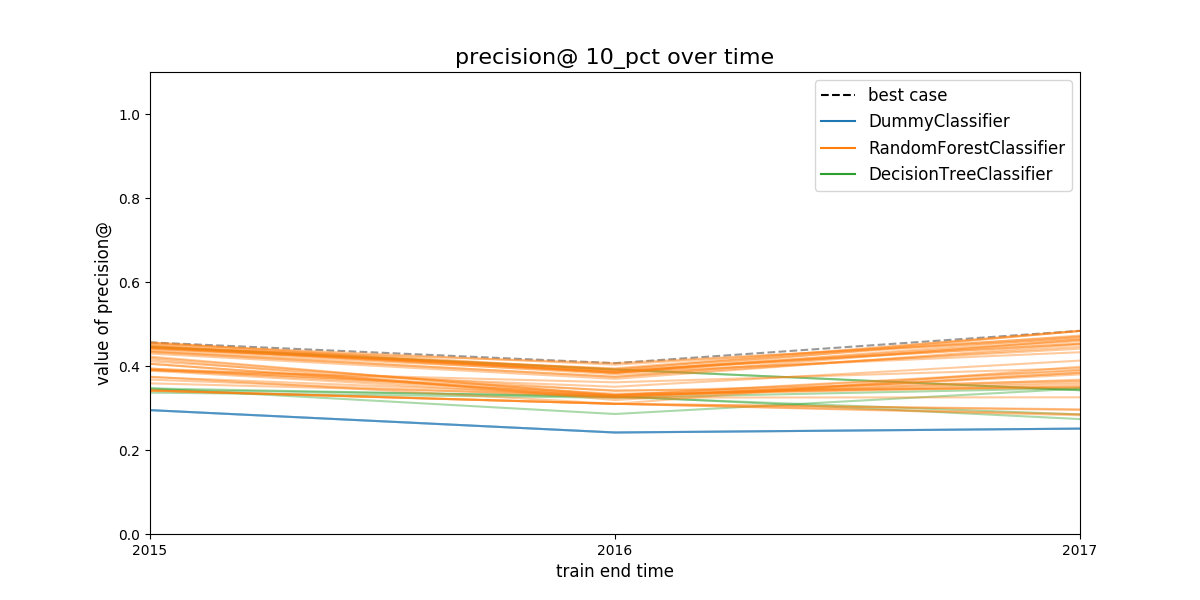Figure. Model group performance over time. In this case the metric show is precision@10%. We didn’t filter out any model group, so the 45 model groups are shown. See discussion above to learn how to plot less model groups. The black dashed line represents the (theoretical) system's performance if we select the best performant model in a every evaluation date. The colored lines represents different model groups. All the model groups that share an algorithm will be colored the same.

Next figure shows the proportion of models that are behind the best model. The distance is measured in percentual points. You could use this plot to filter out more model groups, changing the value of max_from_best in the configuration file. This plot is hard to read, but is very helpful since it shows you the consistency of the model group: How consistently are the model group in a specific range, let's say 20 points, from the best?

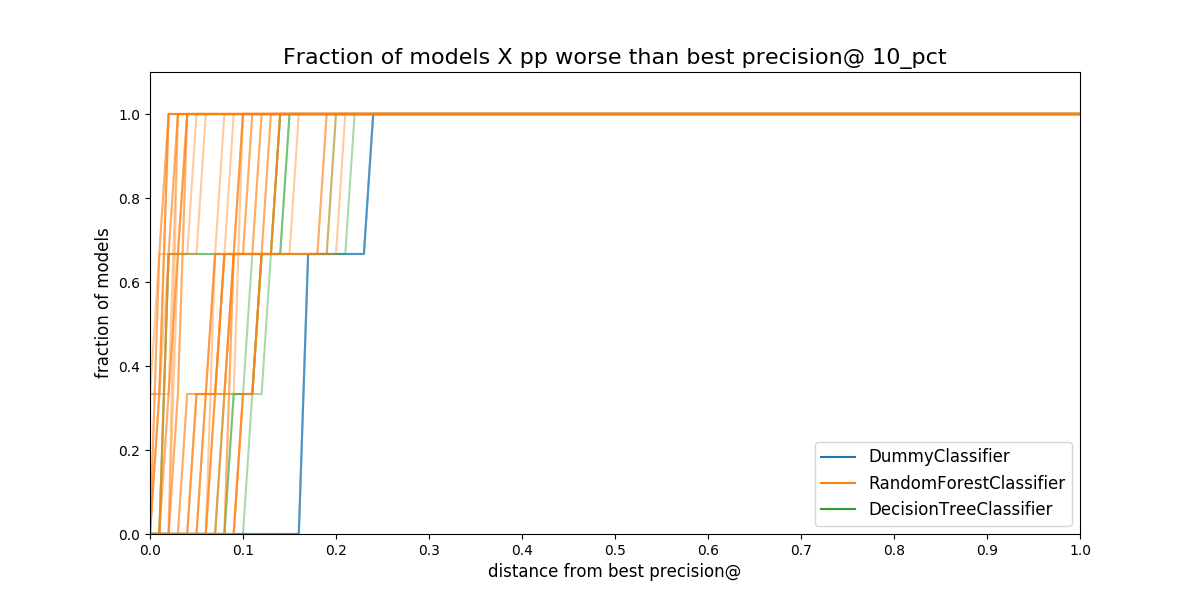Figure. Proportion of *models in a model group that are separated from the best model. The distance is measured in percentual points, i.e. How much less precision at 10 percent of the population compared to the best model in that date.*

In the figure, you can see that the ~60% of the DummyClassifier models are ~18 percentual points below of the best.

Selecting the best rule or strategy for choosing model groups#

In this phase of the audition, you will see what will happen in the next time if you choose your model group with an specific strategy or rule. We call this the regret of the strategies.

We define regret as

Regret Is the difference in performance between the model group you picked and the best one in the next time period.

The next plot show the best model group selected by the strategies specified in the configuration file:

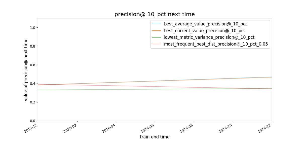Figure. Given a strategy for selecting model groups (in the figure, 4 are shown), What will be the performace of the model group chosen by that strategy in the next evaluation date?

It seems that the strategies best average and best current value select the same model group.

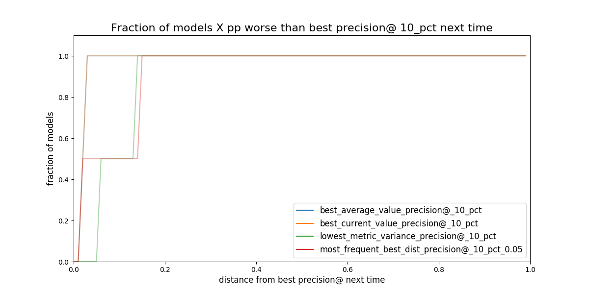Figure. Given a strategy for selecting model groups (in the plot 4 are shown). What will be the distance (*regret) to the best theoretical model in the following evaluation date?*

Obviously, you don’t know the future, but with the available data, if you stick to an a particular strategy, How much you will regret about that decision?

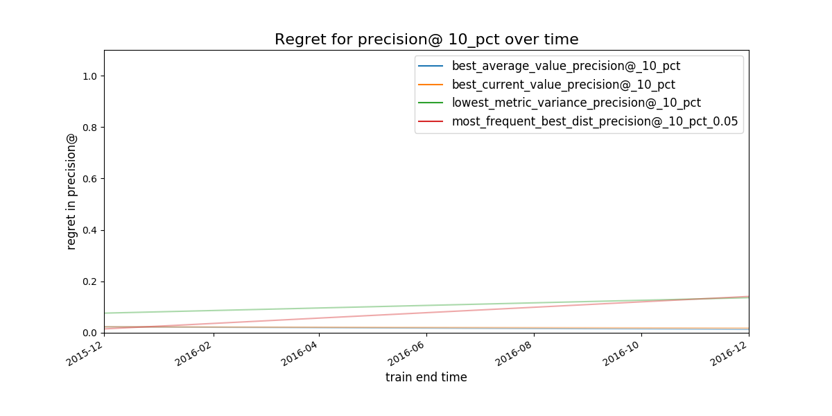Figure. Expected regret for the strategies. The less the better.

The best 3 model groups per strategy will be stored in the file [[file:audition/inspections/results_model_group_ids.json][results_model_group_ids.json]]:

{
    "best_current_value_precision@_10_pct": [39, 30, 9],
    "best_average_value_precision@_10_pct": [39, 9, 29],
    "lowest_metric_variance_precision@_10_pct": [1, 5, 19],
    "most_frequent_best_dist_precision@_10_pct_0.05": [8, 9, 10]
}

The analysis suggests that the best strategies are

select the model groups (39,9,29) which have the best average precision@10% value or,
select the best model group (39,30,9) using precision@10% today and use it for the next time period.

You will note that both strategies share two models groups and differ in one. In the next two sections, we will investigate further those four model groups selected by audition, using the Postmodeling tool set.

Postmodeling: Inspecting the best models closely#

Postmodeling will help you to understand the behaviour orf your selected models (from audition)

As in Audition, we will split the postmodeling process in two parts. The first one is about exploring the model groups filtered by audition, with the objective of select one. The second part is about learning about models in the model group that was selected.

We will setup some parameters in the postmodeling configuration file located at /triage/postmodeling/inspection_postmodeling_config.yaml, mainly where is the audition’s output file located.

# Postmodeling Configuration File

project_path: '/triage' # Project path defined in triage with matrices and models
model_group_id:
  - 39
  - 9
  - 29
  - 30

thresholds: # Thresholds for defining positive predictions
  rank_abs: [50, 100, 250]
  rank_pct: [5, 10, 25]

baseline_query: | # SQL query for defining a baseline for comparison in plots. It needs a metric and parameter
      select g.model_group_id,
             m.model_id,
             extract('year' from m.evaluation_end_time) as as_of_date_year,
             m.metric,
             m.parameter,
             m.value,
             m.num_labeled_examples,
             m.num_labeled_above_threshold,
             m.num_positive_labels
       from test_results.evaluations m
       left join triage_metadata.models g
       using(model_id)
       where g.model_group_id = 1
             and metric = 'precision@'
             and parameter = '10_pct'

max_depth_error_tree: 5 # For error trees, how depth the decision trees should go?
n_features_plots: 10 # Number of features for importances
figsize: [12, 12] # Default size for plots
fontsize: 20 # Default fontsize for plots

Compared to the previous sections, postmodeling is not an automated process (yet). Hence, to do the following part of the tutorial, you need to run jupyter inside bastion as follows:

jupyter-notebook –-ip=0.0.0.0  --port=56406 --allow-root

And then in your browser type¹¹: http://0.0.0.0:56406

Now that you are in a jupyter notebook, type the following:

%matplotlib inline
import matplotlib
#matplotlib.use('Agg')

import triage
import pandas as pd
import numpy as np

from collections import OrderedDict
from triage.component.postmodeling.contrast.utils.aux_funcs import create_pgconn, get_models_ids
from triage.component.catwalk.storage import ProjectStorage, ModelStorageEngine, MatrixStorageEngine
from triage.component.postmodeling.contrast.parameters import PostmodelParameters
from triage.component.postmodeling.contrast.model_evaluator import ModelEvaluator
from triage.component.postmodeling.contrast. model_group_evaluator import ModelGroupEvaluator

After importing, we need to create an sqlalchemy engine for connecting to the database, and read the configuration file.

params = PostmodelParameters('inspection_postmodeling_config.yaml')
engine = create_pgconn('database.yaml')

Postmodeling provides the object ModelGroupEvaluator to compare different model groups.

audited_models_class = ModelGroupEvaluator(tuple(params.model_group_id), engine)

Comparing the audited model groups#

First we will compare the performance of the audited model groups and the baseline over time. First, we will plot precision@10_pct

audited_models_class.plot_prec_across_time(param_type='rank_pct',
                                           param=10,
                                           baseline=True,
                                           baseline_query=params.baseline_query,
                                           metric='precision@',
                                               figsize=params.figsize)

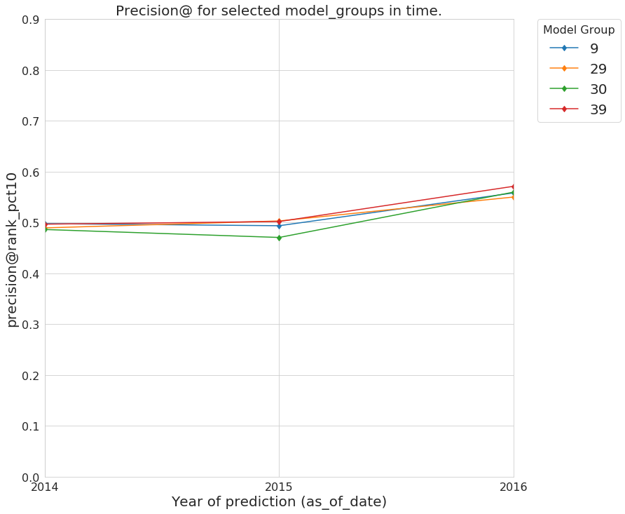Figure. Precision@10% over time from the best performing model groups selected by Audition

and now the recall@10_pct

audited_models_class.plot_prec_across_time(param_type='rank_pct',
                                           param=10,
                                           metric='recall@',
                                           figsize=params.figsize)

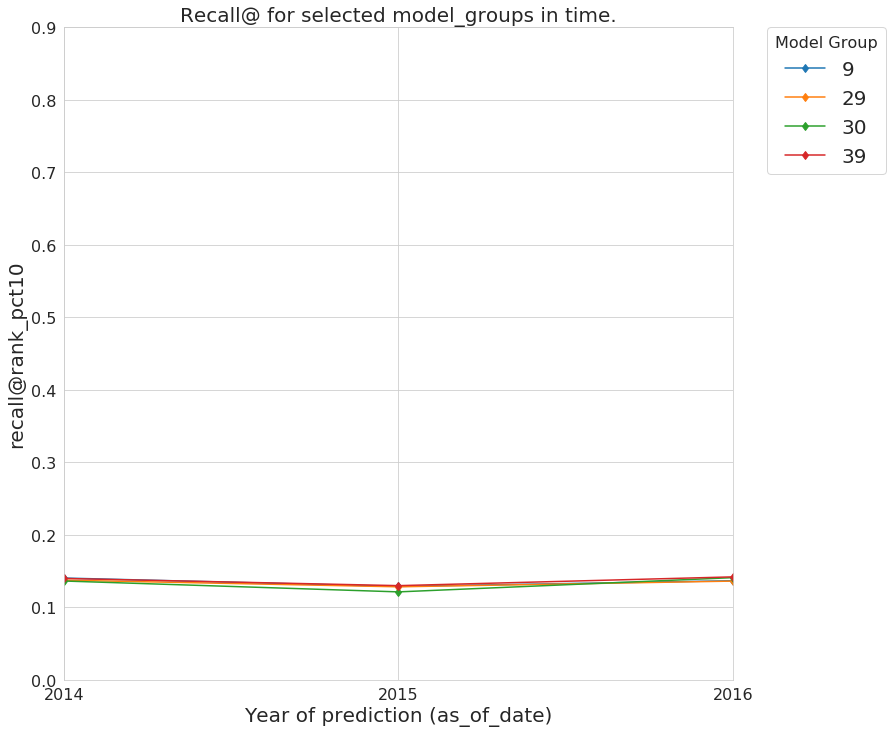Figure. Recall@10% over time from the best performing model groups selected by Audition

All the selected model groups have a very similar performance. Let’s see if they are predicting similar lists of facilities that are at risk of fail an inspection.

audited_models_class.plot_jaccard_preds(param_type='rank_pct',
                                        param=10,
                                        temporal_comparison=True)

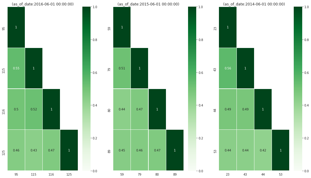Figure. How similar are the model groups’ generated list? We use Jaccard similarity on the predicted lists (length of list 10%) to asses the overlap between lists.

The plot will shows the overlap of the predicted list containing the 10% of the facilities between model groups at each as of date. The lists are at least 50% similar.

Tip

Why the models are not learning the same? You should investigate why is that so. This could lead you to defining new features or some another conclusion about your data, but for this tutorial we will move on.

Going deeper with a model#

Imagine that after a deeper analysis, you decide to choose model group 39

select
    mg.model_group_id,
    mg.model_type,
    mg.hyperparameters,
    array_agg(model_id order by train_end_time) as models
from
    triage_metadata.model_groups as mg
    inner join
    triage_metadata.models
    using (model_group_id)
where model_group_id = 39
group by 1,2,3

model_group_id	model_type	hyperparameters	models
39	sklearn.ensemble.RandomForestClassifier	{"criterion": "gini", "max_features": "sqrt", "n_estimators": 250, "min_samples_split": 10}	{53,89,125}

We will investigate what the particular models are doing. Postmodeling created a ModelEvaluator (similar to the ModelGroupEvaluator) to do this exploration:

models_39 = { f'{model}': ModelEvaluator(39, model, engine) for model in [53,89,125] }

In this tutorial, we will just show some parts of the analysis in the most recent model, but feel free of exploring the behavior of all the models in this model group, and check if you can detect any pattern.

Feature importances

models_39['125'].plot_feature_importances(path=params.project_path,
                                          n_features_plots=params.n_features_plots,
                                          figsize=params.figsize)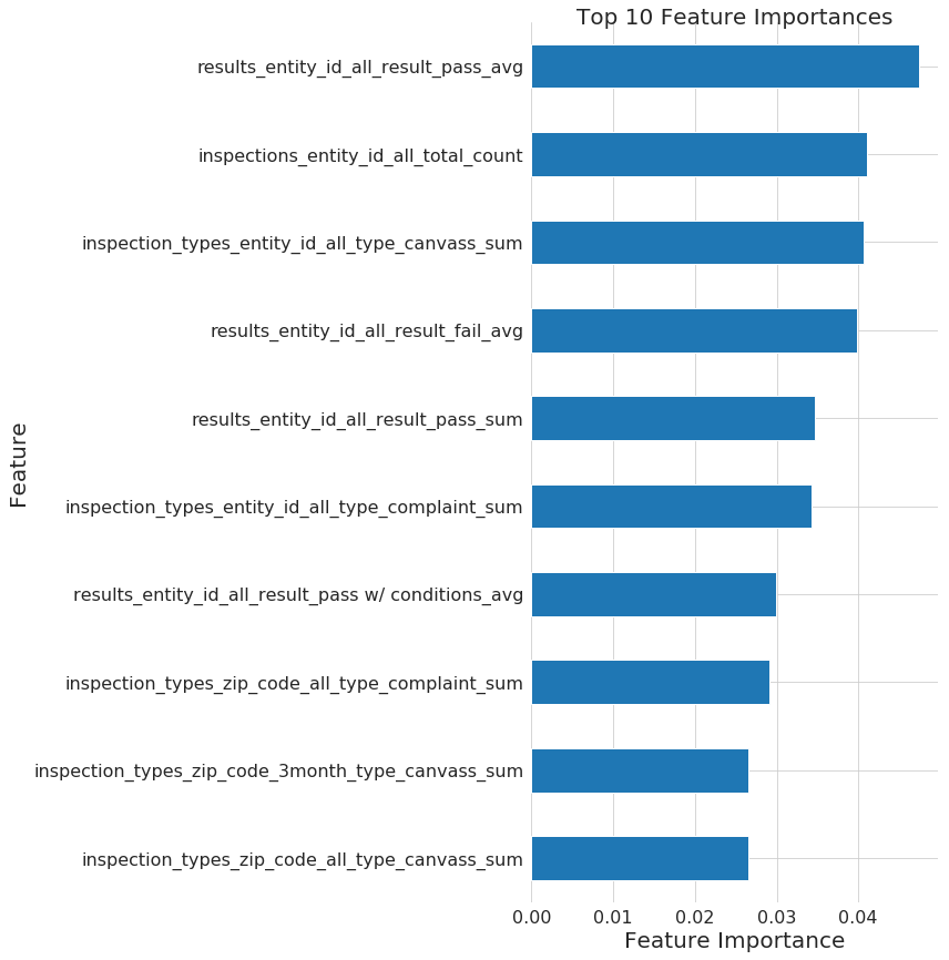

Figure. Top 10 feature importances for de model group 11 at 2016-06-01 (i.e. model 125).

models_39['125'].plot_feature_group_aggregate_importances()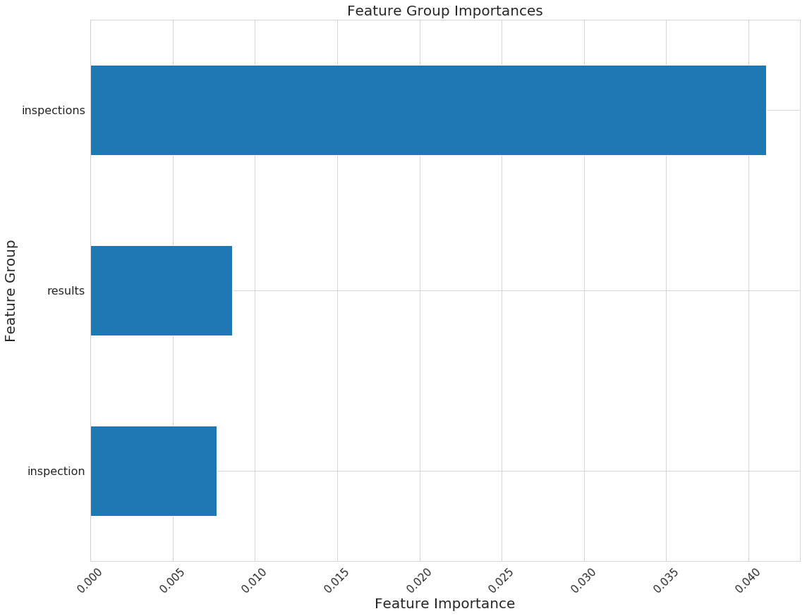

Figure. Feature group “importance” (we are basically taking the max of all the feature importances in a feature group) for the model group 39, model 125.

Our Policy menu

The following plot depicts the behavior of the metrics if you change the length of the facilities predicted at risk (i.e. the $k$ ). This plot is important from the decision making point of view, since it could be used as a policy menu.
```
models_39['125'].plot_precision_recall_n()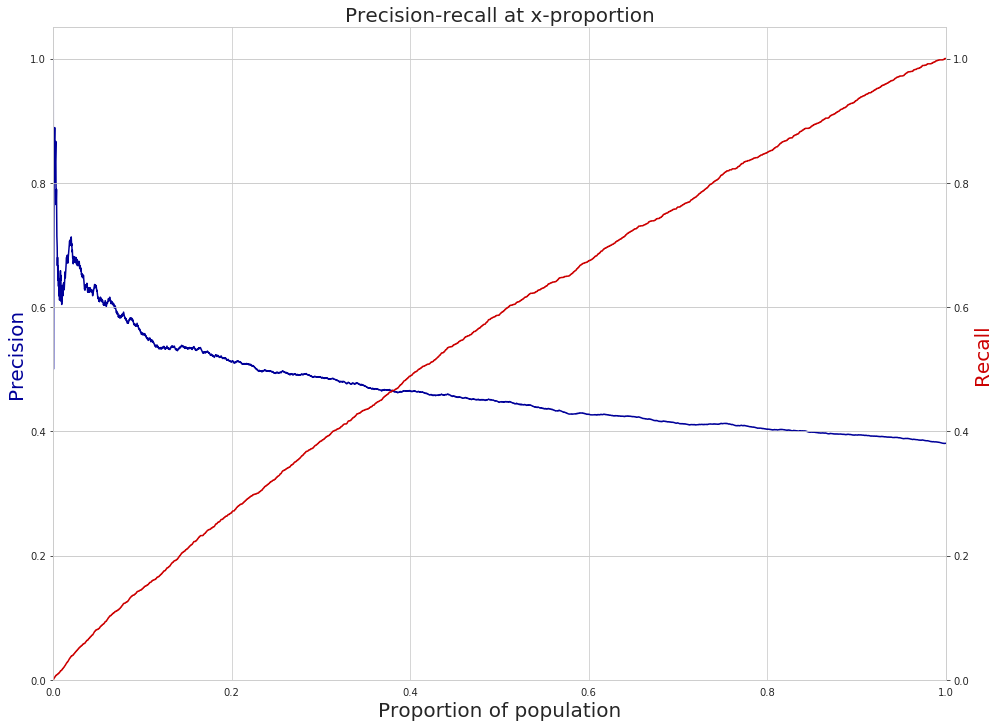
```
Figure. Plot of Precision and Recall over the proportion of the facilities. This plot is used as a "policy menu" since allows you to see how much you will gain if you invest more resources or how much you will sacrifice if you reduce your budget for resources. This is also known as “Rayid plot” at DSaPP.

We selected this model group because it was the best at precision at 10% (i.e. the model group consistently chose facilities will fail inspections at the top 10% of the risk). With the plot above you could decide to double your resources (maybe hiring more inspectors so you could inspect 20% of the facilities) and with this model you will double the detection of facilities that will fail inspections (from ~18% to ~30% in recall) with only a few percent points less of precision ~45% to ~40% (this means that 6 in 10 facilities that the inspectors visit will pass the inspection). You could also go the other way around: if you reduce the length of the list from 10% to 5%, well you will gain a little of precision, but your recall will be ~5%.

Where to go from here#

Ready to get started with your own data? Check out the suggested project workflow for some tips about how to iterate and tune the pipeline for your project.

Want to work through another example? Take a look at our early warning system case study

If you assume a uniform distribution, it will make sense to select facilities at random. ↩
The underlying assumption here is that the City of Chicago is currently doing random selection for the inspections. This is not true (and probably unfair). In a real project, you will setup a real baseline and you will compare your models against it. This baseline could be a rule or a model. ↩
You need to check this! Fortunately, triage allows you to try several options here, so, if you think that this is too high or too low you can change that and fit your needs. ↩
Think about it: we can’t learn the relationship between the features and the label if we don't know the label. ↩
Confused? Check A deeper look at triage for more details. ↩
The formulas are, for precision@k, is the proportion of facilities correctly identified in the top- $k$ facilities ranked by risk:

$$ precision@k = \frac{TP \in k}{k} $$

This is a measure about how efficiently are your system using your resources.

recall@k, in the other hand is the proportion of all the facilities that are risk found in the top- $k$

$$ recall@k = \frac{TP \in k}{TP} $$

recall is a measure about the coverage of your system, i.e. how good is identifying in the top- $k$ the facilities at risk.

One possible variation of this is to only include in the denominator the labeled rows in $k$ . This is the approach used by triage. ↩
We will explore how to one way to tackle this in the advance part of this tutorial. ↩
The flags -no-save-predictions and profile are not necessary but useful. The first one configure triage to not store the predictions (at this stage you don't need them, and you can always could recreate them from the model and the matrix). This will save you execution time. The flag profile stores the execution profile times in a file, so you can check which models or matrices are taking a lot of time on been built. ↩
From a more mathematical point of view: Your data actually reflects the empirical probability: $P(violation|inspected)$ , i.e. the probability of find a violation given that the facility is inspected. But the probability that you want is $P(violation)$ (yes, I know that there are no such things as unconditional probabilities, please bare with me),i.e. the probability that the facility is in violation. ↩
You should see that this assumption is very dangerous in other settings, for example, crime prediction. ↩
This assumes that you are in a GNU/Linux machine, if not (you should reconsider what are you doing with your life) you should change the ip address (0.0.0.0) and use the one from the docker virtual machine. ↩
For some reason, sklearn doesn’t scale the inputs to the Logistic Regression, so we (DSaPP) developed a version that does that. ↩